19 Hypothesis Testing with Simulation

19.1 Objectives

Know and properly use the terminology of a hypothesis test, to include: null hypothesis, alternative hypothesis, test statistic, \(p\)-value, randomization test, one-sided test, two-sided test, statistically significant, significance level, type I error, type II error, false positive, false negative, null distribution, and sampling distribution.
Conduct all four steps of a hypothesis test using randomization.
Discuss and explain the ideas of decision errors, one-sided versus two-sided tests, and the choice of a significance level.

19.2 Homework

19.2.1 Problem 1

Repeat the analysis of the commercial length in the notes. This time use a different test statistic.

ads<-read_csv("data/ads.csv")

ads

## # A tibble: 10 × 2
##    basic premium
##    <dbl>   <dbl>
##  1  6.95    3.38
##  2 10.0     7.8 
##  3 10.6     9.42
##  4 10.2     4.66
##  5  8.58    5.36
##  6  7.62    7.63
##  7  8.23    4.95
##  8 10.4     8.01
##  9 11.0     7.8 
## 10  8.52    9.58

ads <- ads %>%
  pivot_longer(cols=everything(),names_to="channel",values_to = "length")
ads

## # A tibble: 20 × 2
##    channel length
##    <chr>    <dbl>
##  1 basic     6.95
##  2 premium   3.38
##  3 basic    10.0 
##  4 premium   7.8 
##  5 basic    10.6 
##  6 premium   9.42
##  7 basic    10.2 
##  8 premium   4.66
##  9 basic     8.58
## 10 premium   5.36
## 11 basic     7.62
## 12 premium   7.63
## 13 basic     8.23
## 14 premium   4.95
## 15 basic    10.4 
## 16 premium   8.01
## 17 basic    11.0 
## 18 premium   7.8 
## 19 basic     8.52
## 20 premium   9.58

favstats(length~channel,data=ads)

##   channel   min      Q1 median       Q3    max   mean       sd  n missing
## 1   basic 6.950 8.30375  9.298 10.30000 11.016 9.2051 1.396126 10       0
## 2 premium 3.383 5.05250  7.715  7.95975  9.580 6.8592 2.119976 10       0

State the null and alternative hypotheses.

\(H_0\): Null hypothesis. The distribution of length of commercials in premium and basic channels is the same.
\(H_A\): Alternative hypothesis. The distribution of length of commercials in premium and basic channels is different.

Compute a test statistic.

We will use the difference in means so we can use diffmeans() from mosiac.

obs <- diffmean(length~channel,data=ads)
obs

## diffmean 
##  -2.3459

Determine the \(p\)-value.

set.seed(4172)
results <- do(10000)*diffmean(length~shuffle(channel),data=ads)

Next we create a plot of the empirical sampling distribution of the difference of means.

results %>%
  gf_histogram(~diffmean,
               fill="cyan",
               color="black") %>%
  gf_vline(xintercept =obs) %>%
  gf_theme(theme_classic()) %>%
  gf_labs(x="Test statistic")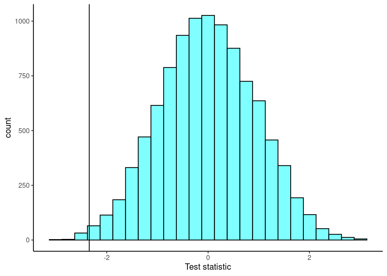

Again, notice it is centered at zero and symmetrical.

prop1(~(diffmean<=obs),data=results)

##  prop_TRUE 
## 0.00459954

The \(p\)-value is much smaller! The test statistic matters in terms of efficiency of the testing procedure.

Draw a conclusion.

Based on our data, if there were really no difference in the distribution of lengths of commercials in 30 minute shows between basic and premium channels then the probability of finding our observed difference of means is 0.005. Since this is less than our significance level of 0.05, we reject the null in favor of the alternative that the basic channel has longer commercials.

19.2.2 Problem 2

Is yawning contagious?. An experiment conducted by the MythBusters, a science entertainment TV program on the Discovery Channel, tested if a person can be subconsciously influenced into yawning if another person near them yawns. 50 people were randomly assigned to two groups: 34 to a group where a person near them yawned (treatment) and 16 to a group where there wasn’t a person yawning near them (control). The following table shows the results of this experiment.

\[ \begin{array}{ccc|cc|c} & & &\textbf{Group} & & \\& & & Treatment & Control & Total \\ &\hline \textbf{Result} & \textit{Yawn} & 10 & 4 & 14 \\ & & \textit{No Yawn} & 24 & 12 & 36\\ &\hline &Total & 34 & 16 & 50 \end{array} \]

The data is in the file “yawn.csv”.

yawn <- read_csv("data/yawn.csv")

glimpse(yawn)

## Rows: 50
## Columns: 2
## $ group   <chr> "treatment", "treatment", "control", "treatment", "treatment",…
## $ outcome <chr> "no_yawn", "no_yawn", "no_yawn", "no_yawn", "no_yawn", "yawn",…

inspect(yawn)

## 
## categorical variables:  
##      name     class levels  n missing
## 1   group character      2 50       0
## 2 outcome character      2 50       0
##                                    distribution
## 1 treatment (68%), control (32%)               
## 2 no_yawn (72%), yawn (28%)

tally(outcome~group,data=yawn,margins = TRUE,format="proportion")

##          group
## outcome     control treatment
##   no_yawn 0.7500000 0.7058824
##   yawn    0.2500000 0.2941176
##   Total   1.0000000 1.0000000

What are the hypotheses?

\(H_0\): Yawning is not contagious, someone in the group yawning does not impact the percentage of the group that yawns. \(p_c - p_t = 0\) or equivalently \(p_c = p_t\) .
\(H_A\): Yawning does have an impact, it is contagious. If someone yawns then you are more likely to yawn. \(p_t > p_c\) or \(p_c - p_t < 0\).

Calculate the observed difference between the yawning rates under the two scenarios. Yes we are giving you the test statistic.

obs <- diffprop(outcome~group,data=yawn)
obs

##    diffprop 
## -0.04411765

Notice that it is negative. If it had been positive, then we would not even need the next step; we would fail to reject the null because the \(p\)-value would be much larger than 0.05. Think about this and make sure you understand.

Estimate the \(p\)-value using randomization.

set.seed(56)
results<-do(10000)*diffprop(outcome~shuffle(group),data=yawn)

prop1(~(diffprop<=obs),data=results)

## prop_TRUE 
## 0.5140486

This is a large \(p\)-value. Notice that if we were doing a two-sided hypothesis test, then doubling the \(p\)-value would exceed 1. Since a \(p\)-value is a probability, this is not possible and so we would report a \(p\)-value of approximately 1. The reason is that the sampling distribution is not symmetrical. We can see this if we plot the hypergeometric distribution for this problem.

gf_dist("hyper",m=16,n=34,k=14) %>%
  gf_theme(theme_classic()) %>%
  gf_refine(scale_x_continuous(breaks=0:14))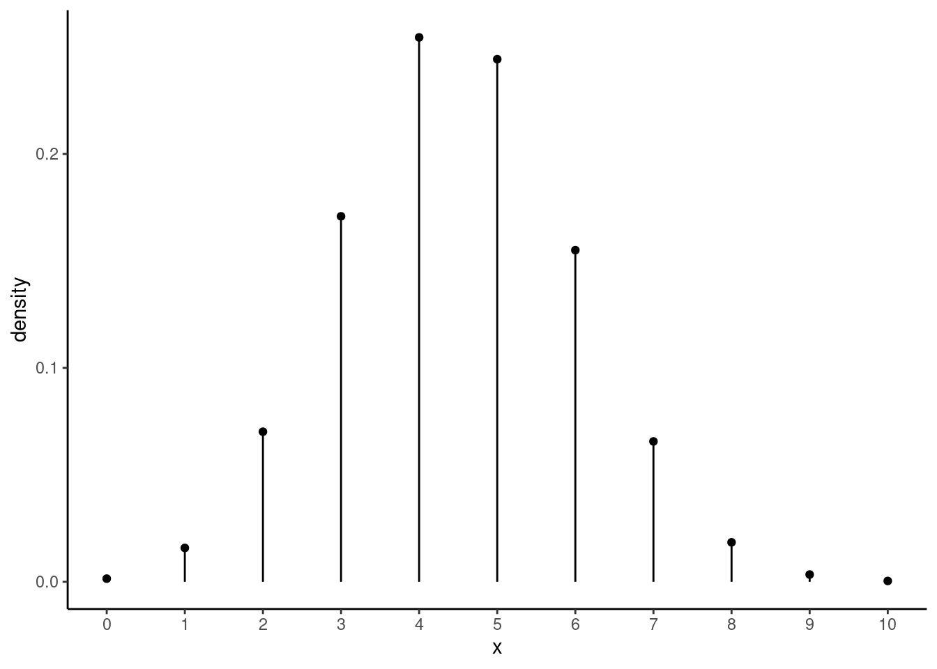

Plot the empirical sampling distribution.

results %>%
  gf_histogram(~diffprop,
               fill="cyan",
               color="black") %>%
  gf_vline(xintercept =obs ) %>%
  gf_theme(theme_classic()) %>%
  gf_labs(x="Test statistic")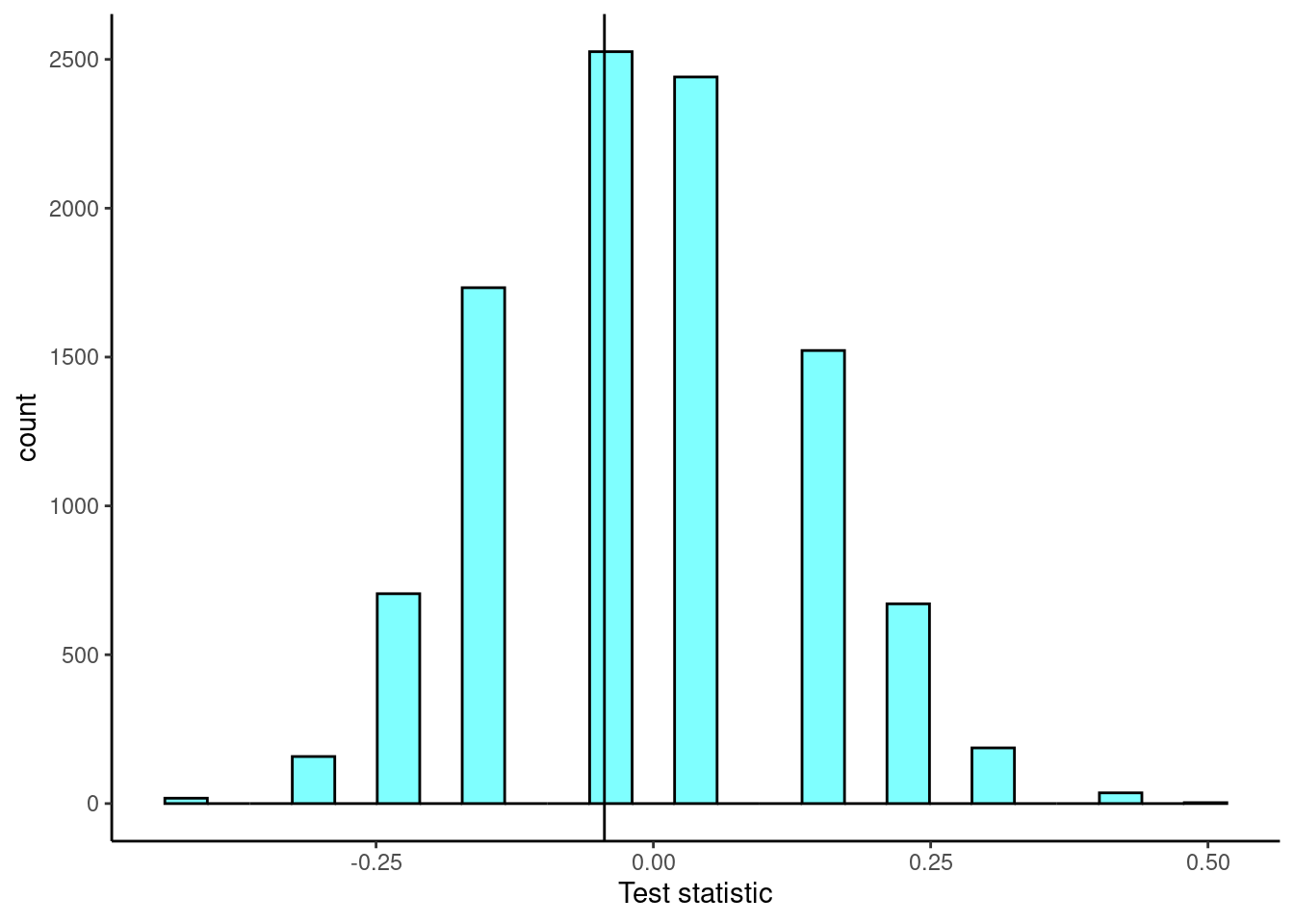

Determine the conclusion of the hypothesis test.

Since \(p\)-value, 0.54, is high, larger than 0.05, we fail to reject the null hypothesis of yawning is not contagious. The data do not provide convincing evidence that people are more likely to yawn if a person near them yawns.

The traditional belief is that yawning is contagious – one yawn can lead to another yawn, which might lead to another, and so on. In this exercise, there was the option of selecting a one-sided or two-sided test. Which would you recommend (or which did you choose)? Justify your answer in 1-3 sentences.

I chose a one-sided test since as a researcher, I thought having someone in the group yawn would lead to more people in that group yawning.

How did you select your level of significance? Explain in 1-3 sentences.

Since there was no clear impact on one type of error being worse than the other, I stayed with the default of 0.05.

Textbook

18 Case Study

20 Hypothesis Testing with Known Distributions