3 Overview of Data Collection Principles
3.1 Objectives
Define and use properly in context all new terminology, to include: population, sample, anecdotal evidence, bias, simple random sample, systematic sample, non-response bias, representative sample, convenience sample, explanatory variable, response variable, observational study, cohort, experiment, randomized experiment, and placebo.
From a description of a research project, be able to describe the population of interest, the generalizability of the study, the explanatory and response variables, whether it is observational or experimental, and determine the type of sample.
In the context of a problem, explain how to conduct a sample for the different types of sampling procedures.
3.2 Homework
3.2.1 Problem 1
Generalizability and causality. Identify the population of interest and the sample in the studies described below. These are the same studies from the previous lesson. Also comment on whether or not the results of the study can be generalized to the population and if the findings of the study can be used to establish causal relationships.
- Researchers collected data to examine the relationship between pollutants and preterm births in Southern California. During the study, air pollution levels were measured by air quality monitoring stations. Specifically, levels of carbon monoxide were recorded in parts per million, nitrogen dioxide and ozone in parts per hundred million, and coarse particulate matter (PM\(_{10}\)) in \(\mu g/m^3\). Length of gestation data were collected on 143,196 births between the years 1989 and 1993, and air pollution exposure during gestation was calculated for each birth. The analysis suggests that increased ambient PM\(_{10}\) and, to a lesser degree, CO concentrations may be associated with the occurrence of preterm births.4
The population of interest is all births. The sample consists of the 143,196 births between 1989 and 1993 in Southern California. If births in this time span can be considered representative of all births, then the results are generalizable to the population of Southern California. The results are likely not generalizable to other geographic areas. Additionally, because the study is observational, the findings cannot be used to establish causal relationships.
- The Buteyko method is a shallow breathing technique developed by Konstantin Buteyko, a Russian doctor, in 1952. Anecdotal evidence suggests that the Buteyko method can reduce asthma symptoms and improve quality of life. In a scientific study to determine the effectiveness of this method, researchers recruited 600 asthma patients aged 18-69 who relied on medication for asthma treatment. These patients were split into two research groups: patients who practiced the Buteyko method and those who did not. Patients were scored on quality of life, activity, asthma symptoms, and medication reduction on a scale from 0 to 10. On average, the participants in the Buteyko group experienced a significant reduction in asthma symptoms and an improvement in quality of life.5
The population is all 18-69 year old people diagnosed with and currently treated for asthma. The sample is the 600 adult patients aged 18-69 years diagnosed with and currently treated for asthma. Since the sample is not random (because it’s voluntary), the results cannot be generalized to the population at large. However, since the study is an experiment, the findings can be used to establish causal relationships.
3.2.2 Problem 2
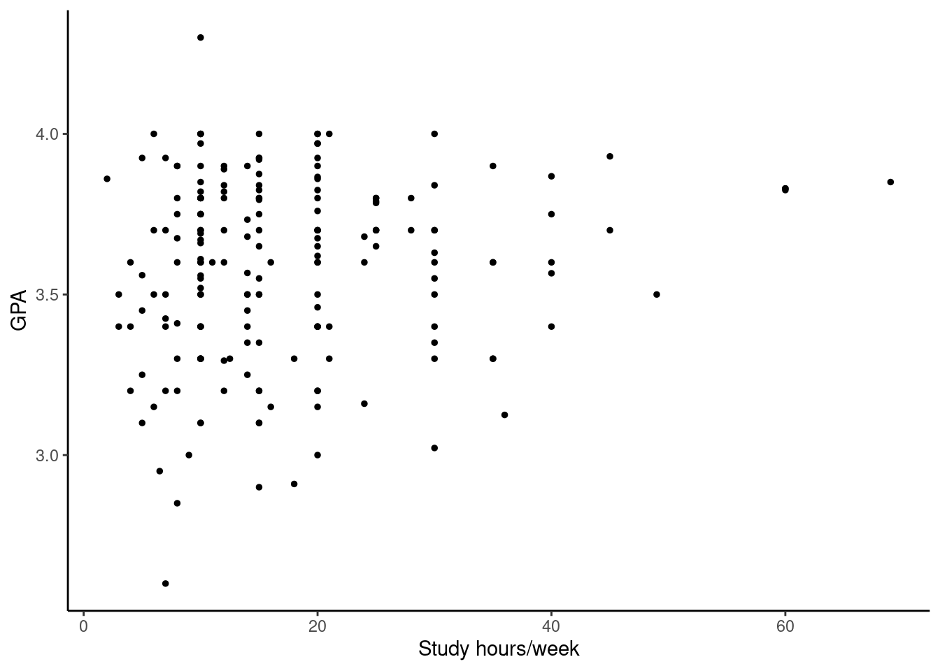
GPA and study time. A survey was conducted on 193 undergraduates who took an introductory statistics course at a private US university in 2012. This survey asked them about their GPA and the number of hours they spent studying per week. The scatterplot below displays the relationship between these two variables.
- What is the explanatory variable and what is the response variable?
The explanatory variable is the number of study hours per week, and the response variable is GPA.
- Describe the relationship between the two variables. Make sure to discuss unusual observations, if any.
There is a somewhat weak positive relationship between the two variables, though the data become more sparse as the number of study hours increases. One respondent reported a GPA above 4.0, which is clearly a data error. Also, there are a few respondents who reported unusually high study hours (60 and 70 hours/week). It should also be noted that the variability in GPA is much higher for students who study less than for those who study more. This also might be due to the fact that there aren’t many respondents who reported a higher number of study hours.
- Is this an experiment or an observational study?
This is an observational study.
- Can we conclude that studying longer hours leads to higher GPAs?
Because this is an observational study, we cannot conclude that there is a causal relationship between the two variables even though there appears to be an association.
3.2.3 Problem 3
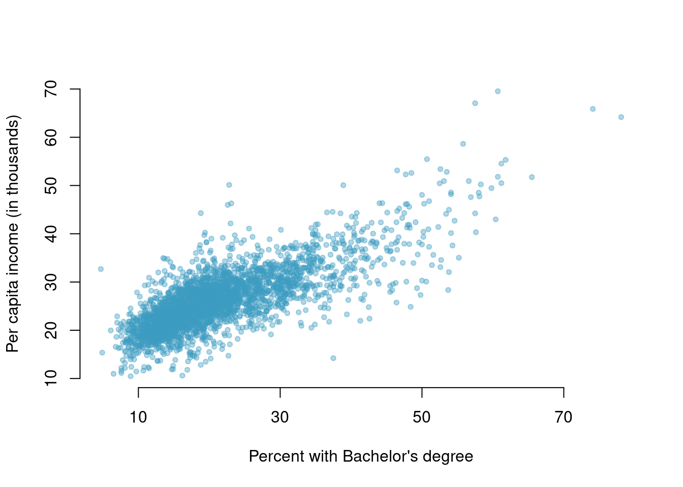
Income and education. The scatterplot below shows the relationship between per capita income (in thousands of dollars) and percent of population with a bachelor’s degree in 3,143 counties in the US in 2010.
- What are the explanatory and response variables?
The explanatory variable is percent of population with a bachelor’s degree and the response variable is per capita income (in thousands of dollars).
- Describe the relationship between the two variables. Make sure to discuss unusual observations, if any.
There is a strong positive linear relationship between the two variables. As the percentage of population with a bachelor’s degree increases, the per capita income increases as well. There are very few counties where more than 60% of the population has a bachelor’s degree and very few counties that have more than $50,000 in per capita income.
- Can we conclude that having a bachelor’s degree increases one’s income?
This is an observational study so we cannot make a causal statement based on the results. However, we can say that having a higher percentage of population with bachelor’s degree is associated with a higher per capita income.