26 Case Study

26.1 Objectives

1. Using R, generate a linear regression model and use it to produce a prediction model.

2. Using plots, check the assumptions of a linear regression model.

26.2 Homework

26.2.1 Problem 1

HFI

Choose another freedom variable and a variable you think would strongly correlate with it. Note: even though some of the variables will appear to be quantitative, they don’t take on enough different values and thus appear to be categorical. So choose with some caution. The openintro package contains the data set hfi. Type ?openintro::hfi in the Console window in RStudio to learn more about the variables.

hfi<-read_csv("data/hfi.csv")

1. Produce a scatterplot of the two variables.

We selected pf_expression_influence as it is a measure of laws and regulations that influence media content. We kept pf_score because it is a measure of personal freedom in a country. Our thought is these should be correlated.

gf_lm(pf_score~pf_expression_influence,data=hfi,color="black") %>%
  gf_theme(theme_bw()) %>%
  gf_point(alpha=0.3) %>%
  gf_labs(title="Personal freedom score versus Control on media",
          x="Laws and regulations that influence media content",
          y="Personal freedom score")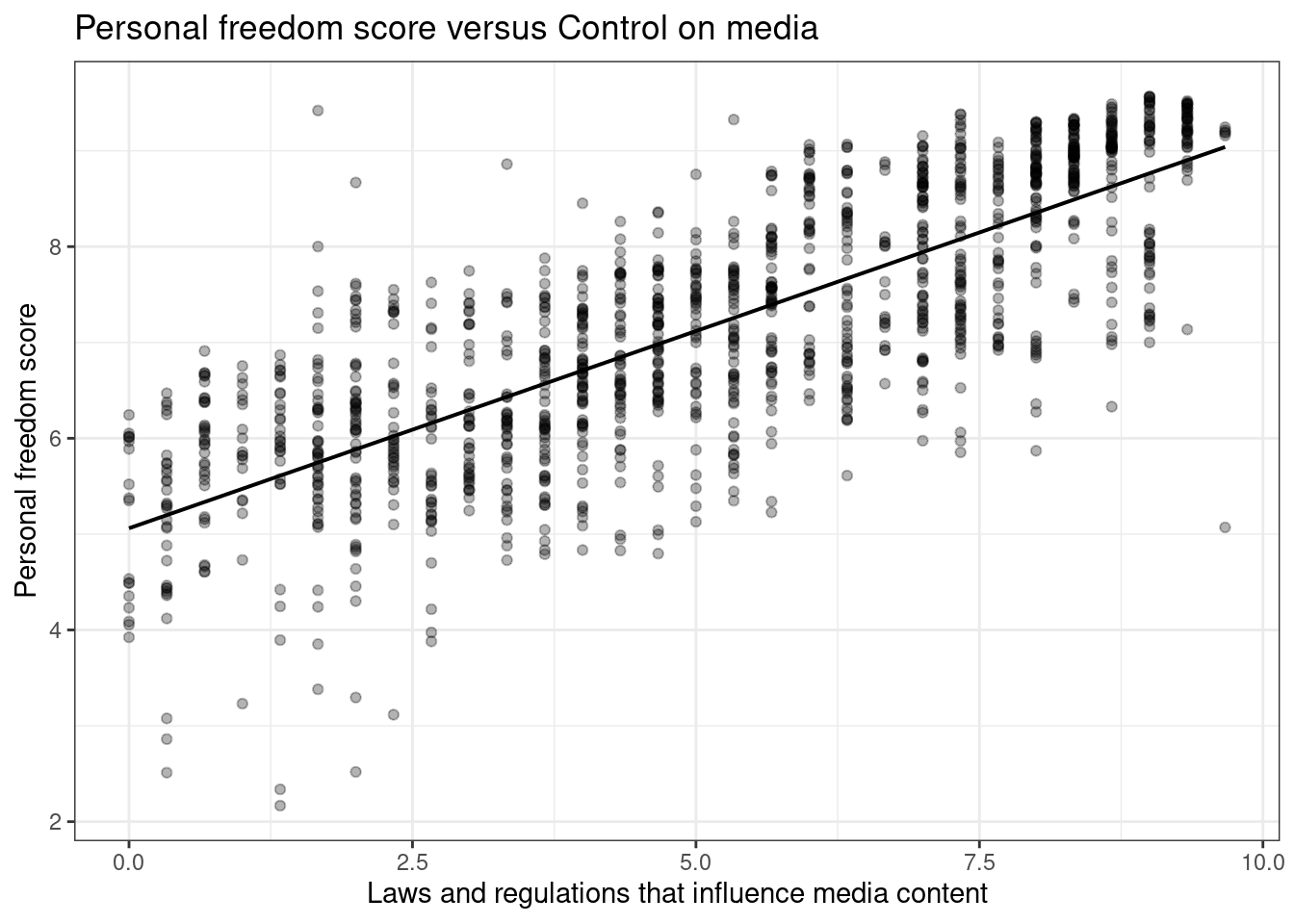

2. Quantify the strength of the relationship with the correlation coefficient.

hfi %>%
  summarise(cor(pf_expression_influence, pf_score, use = "complete.obs"))

## # A tibble: 1 × 1
##   `cor(pf_expression_influence, pf_score, use = "complete.obs")`
##                                                            <dbl>
## 1                                                          0.787

3. Fit a linear model. At a glance, does there seem to be a linear relationship?

m2 <- lm(pf_score ~ pf_expression_influence, data = hfi)

summary(m2)

## 
## Call:
## lm(formula = pf_score ~ pf_expression_influence, data = hfi)
## 
## Residuals:
##     Min      1Q  Median      3Q     Max 
## -3.9688 -0.5830  0.1681  0.5903  3.6730 
## 
## Coefficients:
##                         Estimate Std. Error t value Pr(>|t|)    
## (Intercept)              5.06135    0.05064   99.95   <2e-16 ***
## pf_expression_influence  0.41150    0.00869   47.36   <2e-16 ***
## ---
## Signif. codes:  0 '***' 0.001 '**' 0.01 '*' 0.05 '.' 0.1 ' ' 1
## 
## Residual standard error: 0.8482 on 1376 degrees of freedom
##   (80 observations deleted due to missingness)
## Multiple R-squared:  0.6197, Adjusted R-squared:  0.6195 
## F-statistic:  2243 on 1 and 1376 DF,  p-value: < 2.2e-16

4. How does this relationship compare to the relationship between pf_expression_control and pf_score? Use the \(R^2\) values from the two model summaries to compare. Does your independent variable seem to predict your dependent one better? Why or why not?

   The adjusted \(R^2\) is a little smaller so the fit is not as good.

5. Display the model diagnostics for the regression model analyzing this relationship.

Linearity:

ggplot(data = m2, aes(x = .fitted, y = .resid)) +
  geom_point() +
  geom_hline(yintercept = 0, linetype = "dashed") +
  labs(x="Fitted values",y="Residuals",title="Residual analysis") +
  theme_bw()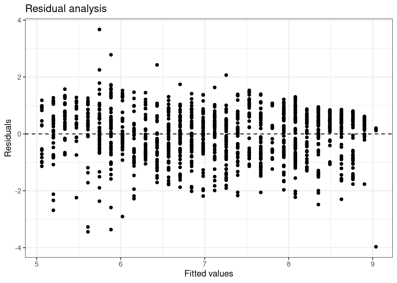

Figure 26.1: Fitted values versus residuals for diagnostics.

There does appear to be some type of fluctuation so the linear model may not be appropriate.

Nearly normal residuals:

ggplot(data = m2, aes(x = .resid)) +
  geom_histogram(binwidth = .4,fill="cyan",color="black") +
  xlab("Residuals") +
  theme_bw()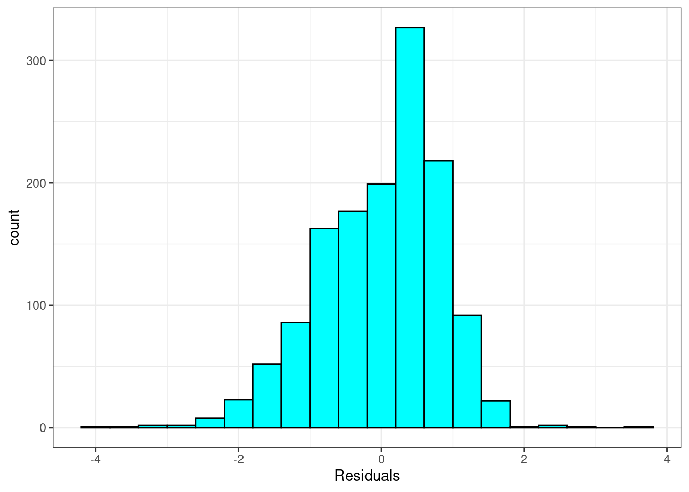

or a normal probability plot of the residuals.

ggplot(data = m2, aes(sample = .resid)) +
  stat_qq() +
  theme_bw() +
  geom_abline(slope=1,intercept = 0)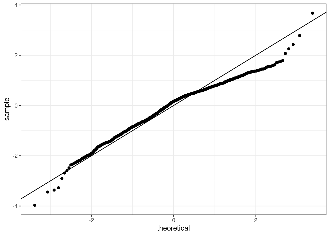

No, the sample is small but it appears the residual are skewed to the left.

Constant variability:

Based on Figure 26.1, the width of the plot seems constant with the exception of some extreme points. The constant variability assumption seems reasonable.

6. Predict the response from your explanatory variable for a value between the median and third quartile. Is this an overestimate or an underestimate, and by how much?

summary(hfi$pf_expression_influence)

##    Min. 1st Qu.  Median    Mean 3rd Qu.    Max.    NA's 
##   0.000   3.000   5.333   5.200   7.333   9.667      80

predict(m2,newdata=data.frame(pf_expression_influence=6))

##       1 
## 7.53036

We thus predict a value of 7.53 for the pf_score.

The observed value is 7.96, an average of 42 data points. We tend to underestimate the observed value.

library(broom)

augment(m2) %>%
   filter(pf_expression_influence==6) %>%
    summarize(ave=mean(pf_score),n=n())

## # A tibble: 1 × 2
##     ave     n
##   <dbl> <int>
## 1  7.96    42

Textbook