28 Linear Regression Inference

28.1 Objectives

Given a simple linear regression model, conduct inference on the coefficients \(\beta_0\) and \(\beta_1\).
Given a simple linear regression model, calculate the predicted response for a given value of the predictor.
Build and interpret confidence and prediction intervals for values of the response variable.

28.2 Homework

28.2.1 Problem 1

We noticed that the 95% prediction interval was much wider than the 95% confidence interval. In words, explain why this is.

The two intervals are describing different parameters. A 95% confidence interval is describing the mean value of the response at a particular value of the predictor. On the other hand, a 95% prediction interval is describing an individual value of the response at a particular value of the predictor. There will be more uncertainty around an individual value than the overall mean.

28.2.2 Problem 2

Beer and blood alcohol content

Many people believe that gender, weight, drinking habits, and many other factors are much more important in predicting blood alcohol content (BAC) than simply considering the number of drinks a person consumed. Here we examine data from sixteen student volunteers at Ohio State University who each drank a randomly assigned number of cans of beer. These students were evenly divided between men and women, and they differed in weight and drinking habits. Thirty minutes later, a police officer measured their blood alcohol content (BAC) in grams of alcohol per deciliter of blood. The data is in the bac.csv file under the data folder.

Create a scatterplot for cans of beer and blood alcohol level.

bac <- read_csv("data/bac.csv")

bac %>%
  gf_point(bac~beers) %>%
  gf_labs(x="Number of cans of beer",y="BAC") %>%
  gf_theme(theme_classic()) %>%
  gf_refine(scale_x_continuous(breaks = c(1,2,3,4,5,6,7,8,9)))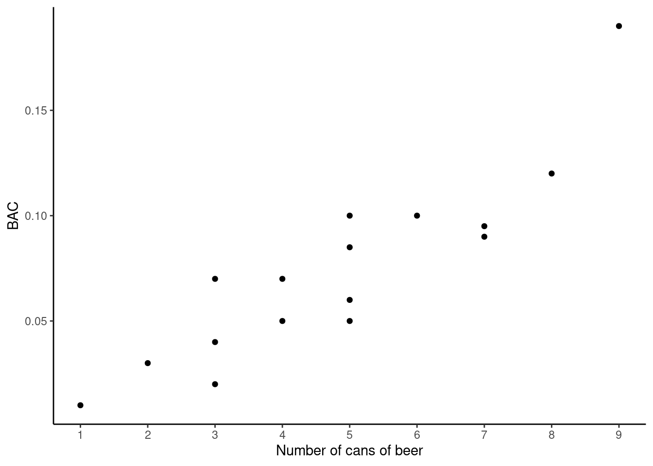

We put BAC as the response since it is more natural to predict BAC from the number of cans of beer consumed. Also notice that the number of cans of beers is really a discrete variable as we can only have whole numbers.

Describe the relationship between the number of cans of beer and BAC.

The relationship appears to be strong, positive and linear. There is one potential outlier, the student who had 9 cans of beer. We will discuss outliers in the next lesson.

Write the equation of the regression line. Interpret the slope and intercept in context.

bac_mod <- lm(bac~beers,data=bac)

summary(bac_mod)

## 
## Call:
## lm(formula = bac ~ beers, data = bac)
## 
## Residuals:
##       Min        1Q    Median        3Q       Max 
## -0.027118 -0.017350  0.001773  0.008623  0.041027 
## 
## Coefficients:
##              Estimate Std. Error t value Pr(>|t|)    
## (Intercept) -0.012701   0.012638  -1.005    0.332    
## beers        0.017964   0.002402   7.480 2.97e-06 ***
## ---
## Signif. codes:  0 '***' 0.001 '**' 0.01 '*' 0.05 '.' 0.1 ' ' 1
## 
## Residual standard error: 0.02044 on 14 degrees of freedom
## Multiple R-squared:  0.7998, Adjusted R-squared:  0.7855 
## F-statistic: 55.94 on 1 and 14 DF,  p-value: 2.969e-06

\[\text{BAC} = -0.0127 + 0.0180 \times \text{beers} \] Slope: For each additional can of beer consumed, the model predicts an additional 0.0180 grams per deciliter BAC on average.

Intercept: Students who don’t have any beer are expected to have a blood alcohol content of -0.0127. This value could be interpreted as how much BAC drops in the time between drinking the beers and when BAC is measured. But it also could be that the intercept is really zero but our estimate is different because of variability in our estimator.

Do the data provide strong evidence that drinking more cans of beer is associated with an increase in blood alcohol? State the null and alternative hypotheses, report the p-value, and state your conclusion.

\(H_0\): The true slope coefficient of number of beers is zero (\(\beta_1 = 0\)).
\(H_a\): The true slope coefficient of number of beers is greater than zero (\(\beta_1 > 0\)).

The p-value for the two-sided alternative hypothesis (\(\beta_1 \neq 0\)) is approximately 0. (Note that this output doesn’t mean the p-value is exactly zero, only that when rounded to four decimal places it is zero.) Therefore the p-value for the one-sided hypothesis will also be very small, it is one half of the p-value reported in the R output. With such a small p-value, we reject \(H_0\) and conclude that the data provide convincing evidence that number of cans of beer consumed and blood alcohol content are positively correlated and the true slope parameter is indeed greater than 0.

Build a 95% confidence interval for the slope and interpret it in the context of your hypothesis test from part d.

We need a lower confidence bound since the alternative is \(\beta_1 > 0\). For a 95% lower confidence bound, we need at 90% confidence interval and then just ignore the upper value.

confint(bac_mod,level=0.9)

##                     5 %        95 %
## (Intercept) -0.03495916 0.009557957
## beers        0.01373362 0.022193906

We are 95% confident that the true value of the slope is greater than 0.014. This bound does not contain 0, so it appears that number of beers and BAC are linearly related in a positive direction. Notice the confidence interval for the intercept does include zero as we discussed above.

Suppose we visit a bar, ask people how many drinks they have had, and also take their BAC. Do you think the relationship between number of drinks and BAC would be as strong as the relationship found in the Ohio State study?

It would probably be weaker. This study had people of very similar ages, and they also had identical drinks. In bars and elsewhere, drinks vary widely in the amount of alcohol they contain.

Predict the average BAC after two beers and build a 90% confidence interval around that prediction.

new_bac <- data.frame(beers=2)
predict(bac_mod, newdata = new_bac, interval = 'confidence',level=0.9)

##          fit         lwr       upr
## 1 0.02322692 0.008308537 0.0381453

Repeat except build a 90% prediction interval and interpret.

predict(bac_mod, newdata = new_bac, interval = 'prediction',level=0.9)

##          fit        lwr        upr
## 1 0.02322692 -0.0157444 0.06219824

We are 90% confident that the BAC of a student who has two beers will be between -.016 and 0.062. Notice that this interval contains an unrealistic level of BAC for the lower limit. If you were briefing this you would make sure to note this. This is because we are using a model based on the normal distribution. A bootstrap may not have this problem. If you truncate the lower level to 0, you have to be careful about claiming 90% coverage.

Plot the data points with a regression line, confidence band, and prediction band.

bac %>%
  gf_point(bac~beers) %>%
  gf_labs(x="Number of cans of beers",y="BAC") %>%
  gf_lm(stat="lm",interval="confidence") %>%
  gf_lm(stat="lm",interval="prediction") %>%
  gf_theme(theme_classic()) %>%
  gf_refine(scale_x_continuous(breaks = c(1,2,3,4,5,6,7,8,9)))

## Warning: Using the `size` aesthetic with geom_ribbon was deprecated in ggplot2 3.4.0.
## ℹ Please use the `linewidth` aesthetic instead.
## This warning is displayed once every 8 hours.
## Call `lifecycle::last_lifecycle_warnings()` to see where this warning was
## generated.

## Warning: Using the `size` aesthetic with geom_line was deprecated in ggplot2 3.4.0.
## ℹ Please use the `linewidth` aesthetic instead.
## This warning is displayed once every 8 hours.
## Call `lifecycle::last_lifecycle_warnings()` to see where this warning was
## generated.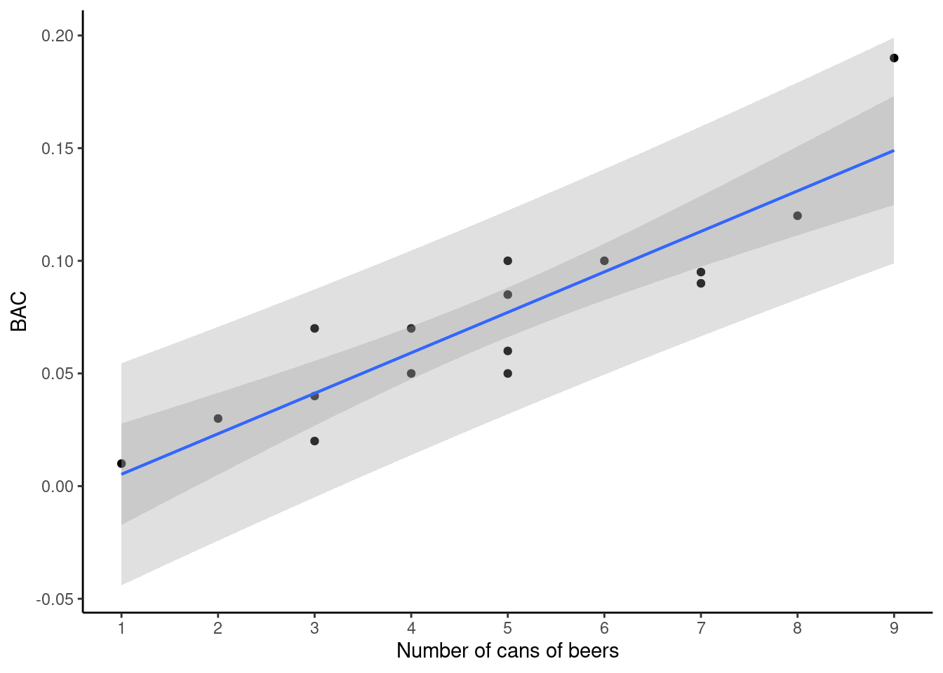

28.2.3 Problem 3

Suppose I build a regression fitting a response variable to one predictor variable. I build a 95% confidence interval on \(\beta_1\) and find that it contains 0, meaning that a slope of 0 is feasible. Does this mean that the response and the predictor are independent?

No. It merely means that my best guess is that the two variables are linearly uncorrelated. They could be related another way (quadratically, for example), but still result in an estimated slope close to 0.

Textbook

27 Linear Regression Basics

29 Linear Regression Diagnostics