21 Hypothesis Testing with the Central Limit Theorem
21.1 Objectives
Explain the central limit theorem and when it can be used for inference.
Conduct hypothesis tests of a single mean and proportion using the CLT and
R.Explain how the \(t\) distribution relates to the normal distribution, where it is used, and how changing parameters impacts the shape of the distribution.
21.2 Homework
21.2.1 Problem 1
Suppose we roll a fair six-sided die and let \(X\) be the resulting number. The distribution of \(X\) is discrete uniform. (Each of the six discrete outcomes is equally likely.)
- Suppose we roll the fair die 5 times and record the value of \(\bar{X}\), the mean of the resulting rolls. Under the central limit theorem, what should be the distribution of \(\bar{X}\)?
The mean of \(X\) is 3.5 and the variance of \(X = \frac{(b-a+1)^2-1}{12} = \frac{35}{12}\) is 2.9167. So, \[ \bar{X}\overset{approx}{\sim}\textsf{Norm}(3.5,0.764) \]
- Simulate this process in
R. Plot the resulting empirical distribution of \(\bar{X}\) and report the mean and standard deviation of \(\bar{X}\). Was it what you expected?
(HINT: You can simulate a die roll using the sample function. Be careful and make sure you use it properly.)
results %>%
   gf_histogram(~mean,fill="cyan",color="black") %>%
   gf_theme(theme_classic()) %>%
   gf_labs(x="Test statistic")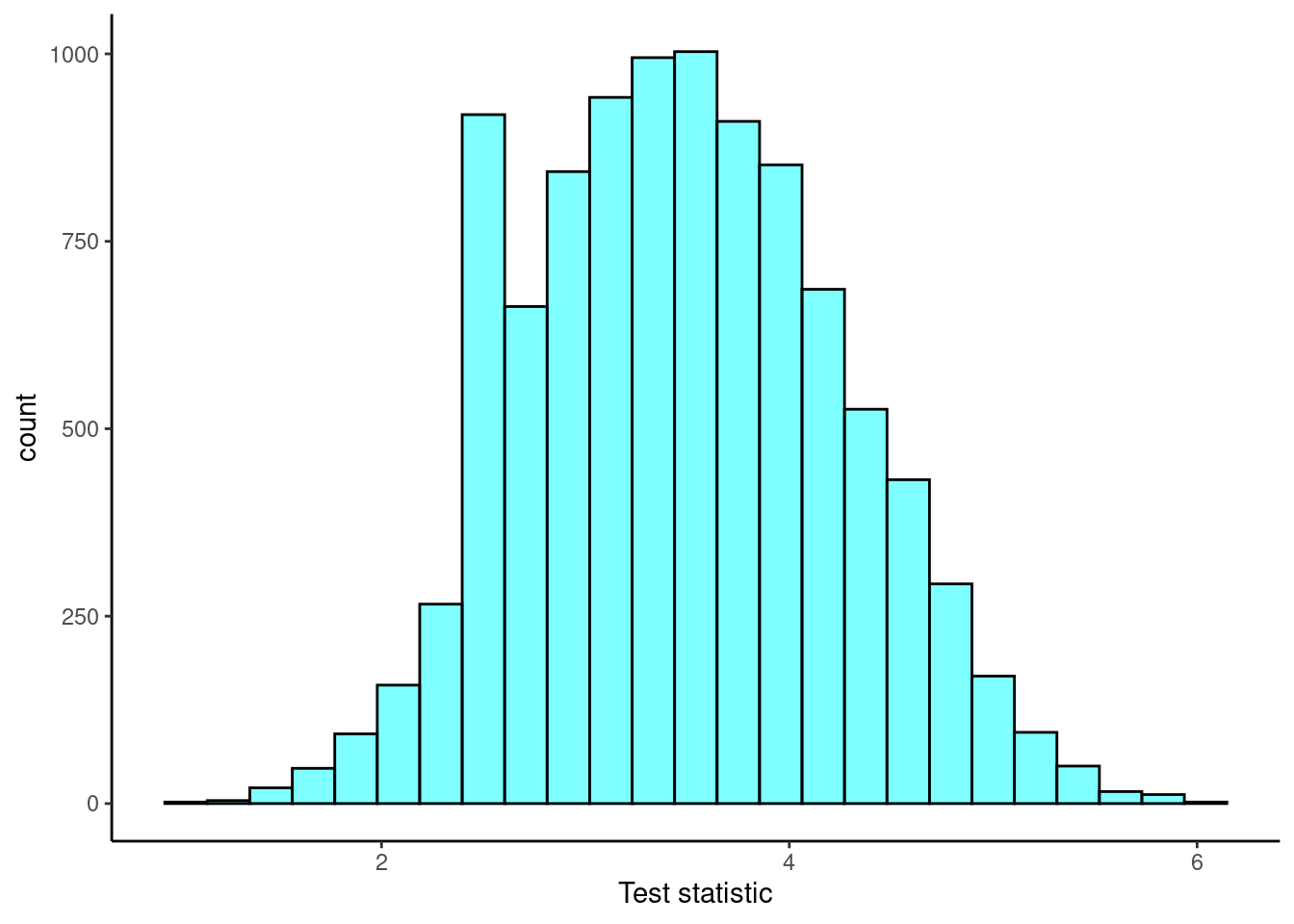
favstats(~mean,data=results)## min Q1 median Q3 max mean sd n missing
## 1 3 3.6 4 6 3.51278 0.772254 10000 0It appears to be roughly normally distributed with the mean and standard deviation we expected.
- Repeat parts a) and b) for \(n=20\) and \(n=50\). Describe what you notice. Make sure all three plots are plotted on the same \(x\)-axis scale. You can use facets if you combine your data into one
tibble.
When \(n=20\): \[ \bar{X}\overset{approx}{\sim}\textsf{Norm}(3.5,0.382) \]
results2<-do(10000)*mean(sample(6,20,replace=T))
results2 %>%
   gf_histogram(~mean,fill="cyan",color="black") %>%
   gf_theme(theme_classic()) %>%
   gf_labs(x="Test statistic")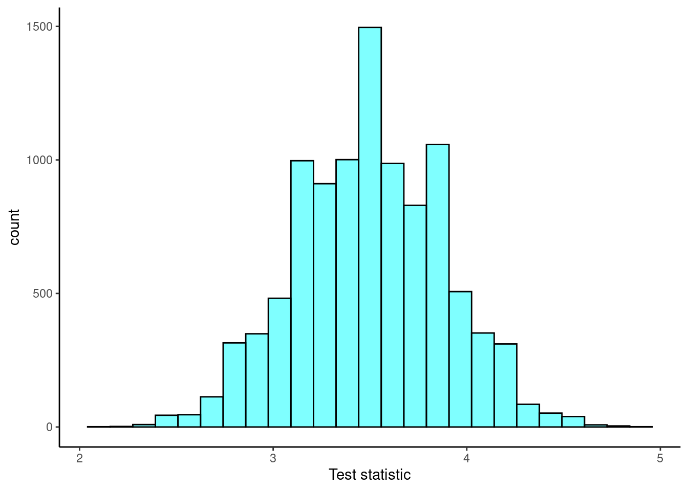
favstats(~mean,data=results2)## min Q1 median Q3 max mean sd n missing
## 2.15 3.25 3.5 3.75 4.95 3.49896 0.3828754 10000 0When \(n=50\): \[ \bar{X}\overset{approx}{\sim}\textsf{Norm}(3.5,0.242) \]
results3<-do(10000)*mean(sample(6,50,replace=T))
results3 %>%
   gf_histogram(~mean,fill="cyan",color="black") %>%
   gf_theme(theme_classic()) %>%
   gf_labs(x="Test statistic")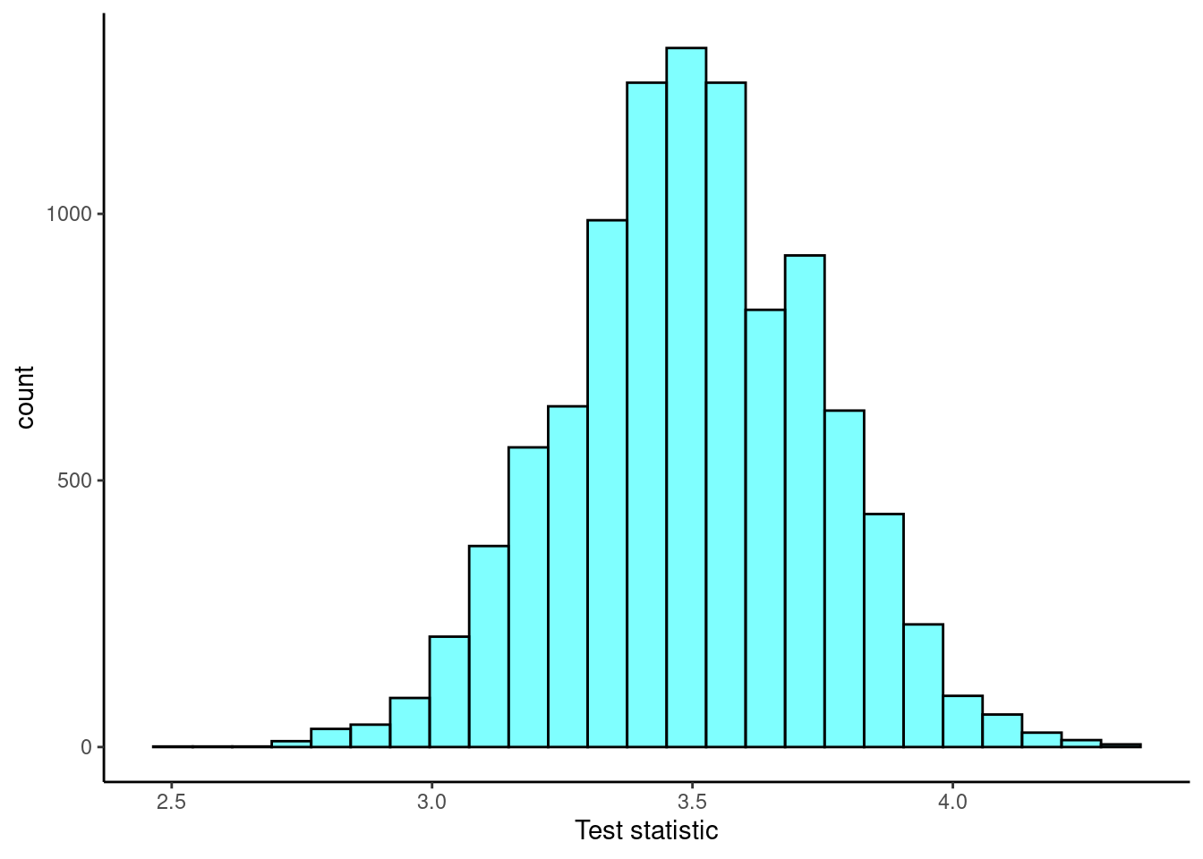
favstats(~mean,data=results3)## min Q1 median Q3 max mean sd n missing
## 2.54 3.34 3.5 3.66 4.36 3.49852 0.2423665 10000 0Now let’s put them all together to make it easier to compare.
final_results %>%
   gf_dhistogram(~mean|n,fill="cyan",color="black") %>%
   gf_theme(theme_classic()) %>%
   gf_labs(x="Test statistic")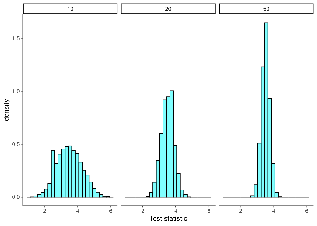
##      mean        sd  n
## 1 3.51278 0.7722540 10
## 2 3.49896 0.3828754 20
## 3 3.49852 0.2423665 50
All results were as expected. As \(n\) increased, the variance of the sample mean decreased.
21.2.2 Problem 2
The nutrition label on a bag of potato chips says that a one ounce (28 gram) serving of potato chips has 130 calories and contains ten grams of fat, with three grams of saturated fat. A random sample of 35 bags yielded a sample mean of 134 calories with a standard deviation of 17 calories. Is there evidence that the nutrition label does not provide an accurate measure of calories in the bags of potato chips? The conditions necessary for applying the normal model have been checked and are satisfied.
The question has been framed in terms of two possibilities: the nutrition label accurately lists the correct average calories per bag of chips or it does not, which may be framed as a hypothesis test.
- Write the null and alternative hypothesis.
\(H_0\): The average is listed correctly. \(\mu = 130\)
\(H_A\): The nutrition label is incorrect. \(\mu \neq 130\)
- What level of significance are you going to use?
I am going to use \(\alpha = 0.05\).
- What is the distribution of the test statistic \({\bar{X}-\mu\over S/\sqrt{n}}\)? Calculate the observed value.
The distribution of the test statistic is \(t\) with 34 degrees of freedom.
The observed average is \(\bar{x} = 134\) and the standard error may be calculated as \(SE = \frac{17}{\sqrt{35}} = 2.87\).
We can compute a test statistic as the t score:
\[ t = \frac{134 - 130}{2.87} = 1.39 \]
- Calculate a \(p\)-value.
The upper-tail area is 0.0823,
pt(1.39,34,lower.tail = F)## [1] 0.08678153or
1-pt(1.39,34)## [1] 0.08678153so the \(p\)-value is \(2 \times 0.0823 = 0.1646\).
- Draw a conclusion.
Since the \(p\)-value is larger than 0.05, we do not reject the null hypothesis. That is, there is not enough evidence to show the nutrition label has incorrect information.
21.2.2.1 Extra material
If we had used a normal model based on the CLT our \(p\)-value would have been close to the value from the \(t\) because our sample size is large.
pnorm(1.39,lower.tail = F)## [1] 0.0822644421.2.3 Problem 3
Find the \(p\)-value. An independent random sample is selected from an approximately normal population with an unknown standard deviation. Find the \(p\)-value for the given set of hypotheses and \(T\) test statistic. Also determine if the null hypothesis would be rejected at \(\alpha = 0.05\).
- \(H_{A}: \mu > \mu_{0}\), \(n = 11\), \(T = 1.91\)
1-pt(1.91,10)## [1] 0.04260244The \(p\)-value is less than 0.05, reject the null hypothesis.
- \(H_{A}: \mu < \mu_{0}\), \(n = 17\), \(T = - 3.45\)
pt(-3.45,16)## [1] 0.001646786The \(p\)-value is less than 0.05, reject the null hypothesis.
- \(H_{A}: \mu \ne \mu_{0}\), \(n = 7\), \(T = 0.83\)
2*(1-pt(0.83,6))## [1] 0.4383084The \(p\)-value is greater than 0.05, fail to reject the null hypothesis.
- \(H_{A}: \mu > \mu_{0}\), \(n = 28\), \(T = 2.13\)
1-pt(2.13,27)## [1] 0.02121769The \(p\)-value is less than 0.05, reject the null hypothesis.
21.2.4 Problem 4
In this lesson, we have used the expression degrees of freedom a lot. What does this expression mean? When we have sample of size \(n\), why are there \(n-1\) degrees of freedom for the \(t\) distribution? Give a short concise answer (about one paragraph). You will likely have to do a little research on your own.
Answers will vary. One possible explanation is that the degrees of freedom represents the number of independent pieces of information. For example, you’ll notice that in order to get an unbiased estimate of \(\sigma^2\), we have to divide by \(n-1\). This is because in order to estimate \(\sigma^2\), we need to first estimate \(\mu\), which is done by obtaining the sample mean. Once we know the sample mean, we only have \(n-1\) pieces of independent information. For example, suppose we have a sample of size 10, and we know the sample mean. Once we are given the first 9 observations, we know exactly what the 10th observation must be.
21.2.5 Problem 5
Deborah Toohey is running for Congress, and her campaign manager claims she has more than 50% support from the district’s electorate. Ms. Toohey’s opponent claimed that Ms. Toohey has less than 50%. Set up a hypothesis test to evaluate who is right.
- Should we run a one-sided or two-sided hypothesis test?
We should run a two-sided. She could be greater than 50% regardless of what the opponent claims.
- Write the null and alternative hypothesis.
\(H_0\): Ms. Toohey’s support is 50%. \(p = 0.50\).
\(H_A\): Ms. Toohey’s support is either above or below 50%. \(p \neq 0.50\).
- What level of significance are you going to use?
\(\alpha = 0.05\)
- What are the assumptions of this test?
The observations are independent.
There are at least 10 votes for and 10 against.
Because this is a simple random sample that includes fewer than 10% of the population, the observations are independent. In a single proportion hypothesis test, the success-failure condition is checked using the null proportion, \(p_0=0.5\): \(np_0 = n(1-p_0) = 500\times 0.5 = 250 \geq 10\). With these conditions verified, the normal model based on the CLT may be applied to \(\hat{p}\).
- Calculate the test statistic.
A newspaper collects a simple random sample of 500 likely voters in the district and estimates Toohey’s support to be 52%.
The test statistic is \(\bar{x}=0.52\)
- Calculate a \(p\)-value.
Based on the normal model, we can compute a one-sided \(p\)-value and then double to get the correct \(p\)-value.
The standard error can be computed. The null value is used again here, because this is a hypothesis test for a single proportion with the specified value for the probability of success.
\[SE = \sqrt{\frac{p_0\times (1-p_0)}{n}} = \sqrt{\frac{0.5\times (1-0.5)}{500}} = 0.022\]
2*pnorm(.52,mean=.5,sd=0.022,lower.tail = FALSE)## [1] 0.3633021- Draw a conclusion.
Because the \(p\)-value is larger than 0.05, we do not reject the null hypothesis, and we do not find convincing evidence to support the campaign manager’s claim.