32 Logistic Regression
32.1 Objectives
Using
R, conduct logistic regression, interpret the output, and perform model selection.Write the logistic regression model and predict outputs for given inputs.
Find confidence intervals for parameter estimates and predictions.
Create and interpret a confusion matrix.
32.2 Homework Problems
32.2.1 Problem 1
Possum classification
Let’s investigate the possum data set again. This time we want to model a binary outcome variable. As a reminder, the common brushtail possum of the Australia region is a bit cuter than its distant cousin, the American opossum. We consider 104 brushtail possums from two regions in Australia, where the possums may be considered a random sample from the population. The first region is Victoria, which is in the eastern half of Australia and traverses the southern coast. The second region consists of New South Wales and Queensland, which make up eastern and northeastern Australia.
We use logistic regression to differentiate between possums in these two regions. The outcome variable, called pop, takes value Vic when a possum is from Victoria and other when it is from New South Wales or Queensland. We consider five predictors: sex, head_l, skull_w, total_l, and tail_l.
- Explore the data by making histograms of the quantitative variables, and bar charts of the discrete variables. Are there any outliers that are likely to have a very large influence on the logistic regression model?
possum <- read_csv("data/possum.csv") %>%
  select(pop,sex,head_l,skull_w,total_l,tail_l) %>%
  mutate(pop=factor(pop),sex=factor(sex))
inspect(possum)##
## categorical variables:
## name class levels n missing distribution
## 1 pop factor 2 104 0 other (55.8%), Vic (44.2%)
## 2 sex factor 2 104 0 m (58.7%), f (41.3%)
##
## quantitative variables:
## name class min Q1 median Q3 max mean sd n missing
## 1 head_l numeric 82.5 90.675 92.80 94.725 103.1 92.60288 3.573349 104 0
## 2 skull_w numeric 50.0 54.975 56.35 58.100 68.6 56.88365 3.113426 104 0
## 3 total_l numeric 75.0 84.000 88.00 90.000 96.5 87.08846 4.310549 104 0
## 4 tail_l numeric 32.0 35.875 37.00 38.000 43.0 37.00962 1.959518 104 0
possum %>%
  gf_props(~pop,fill="cyan",color="black") %>%
  gf_theme(theme_bw()) %>%
  gf_labs(x="Population")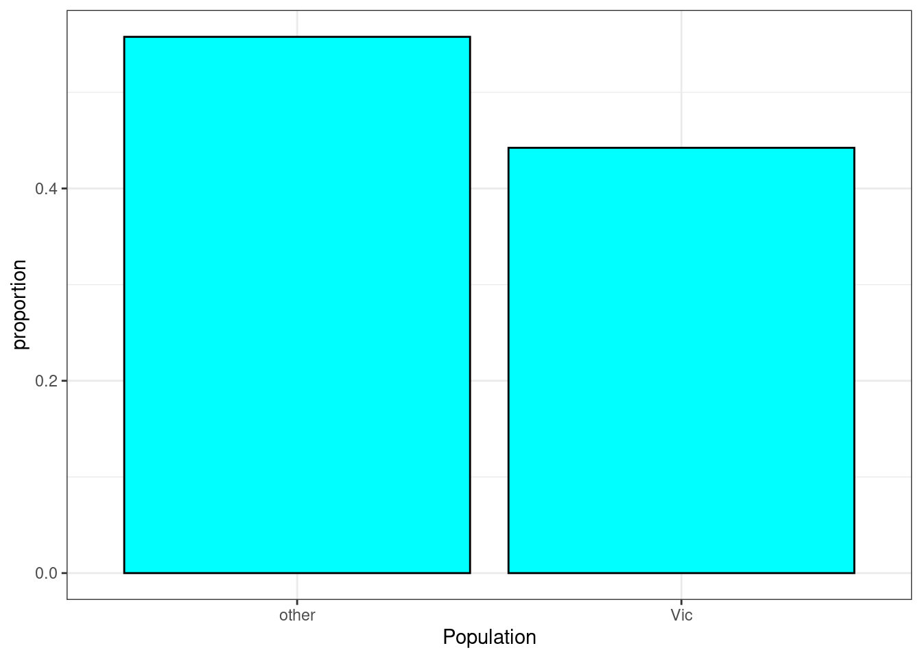
possum %>%
  gf_props(~sex,fill="cyan",color="black") %>%
  gf_theme(theme_bw()) %>%
  gf_labs(x="Gender")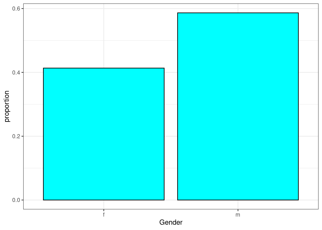
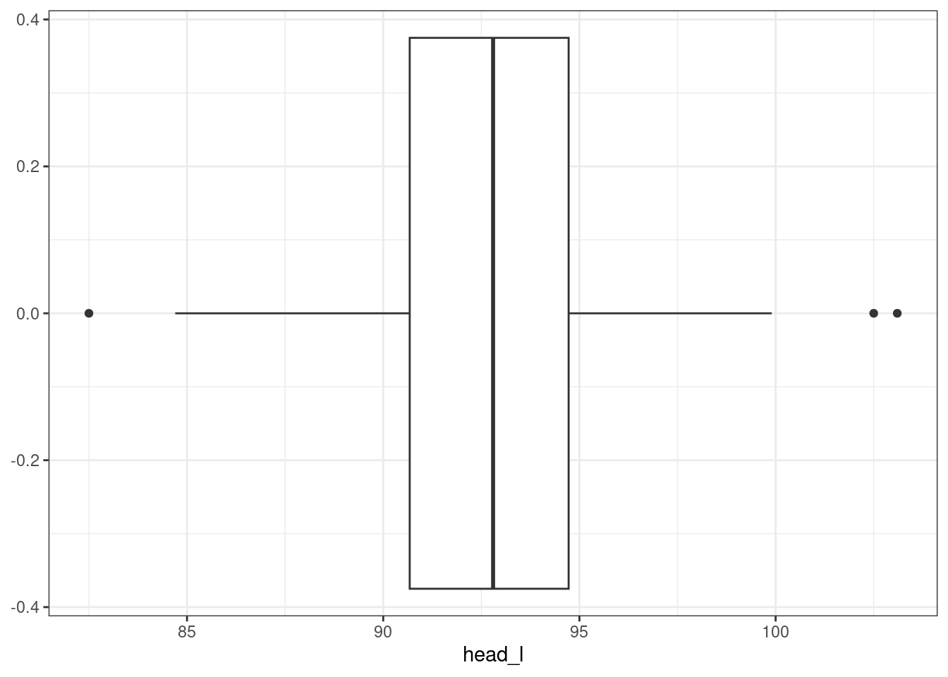
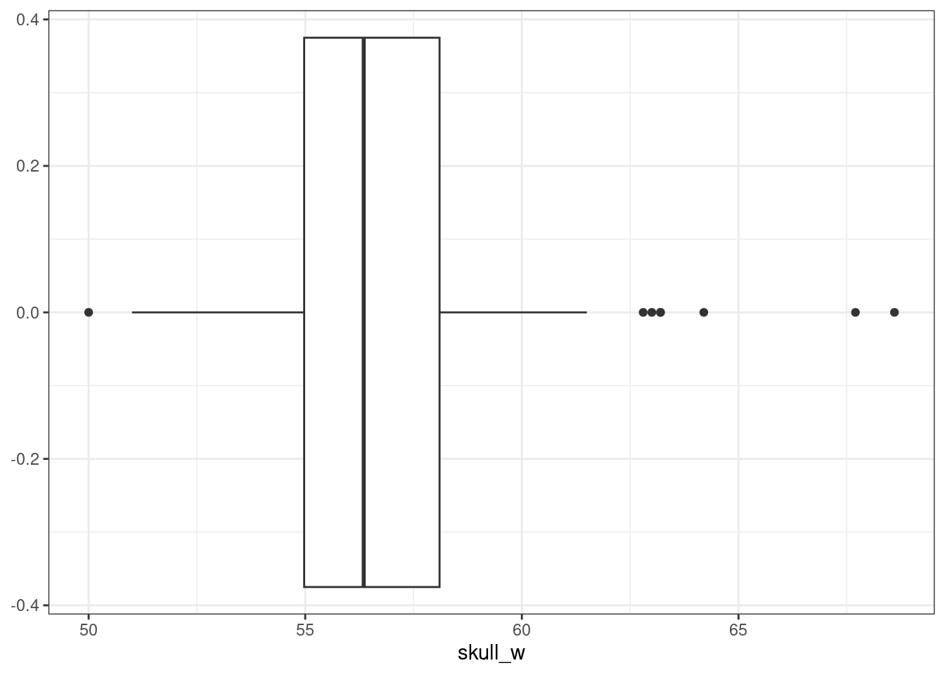
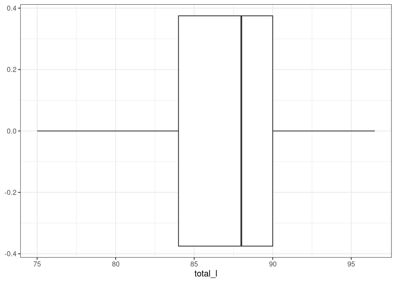
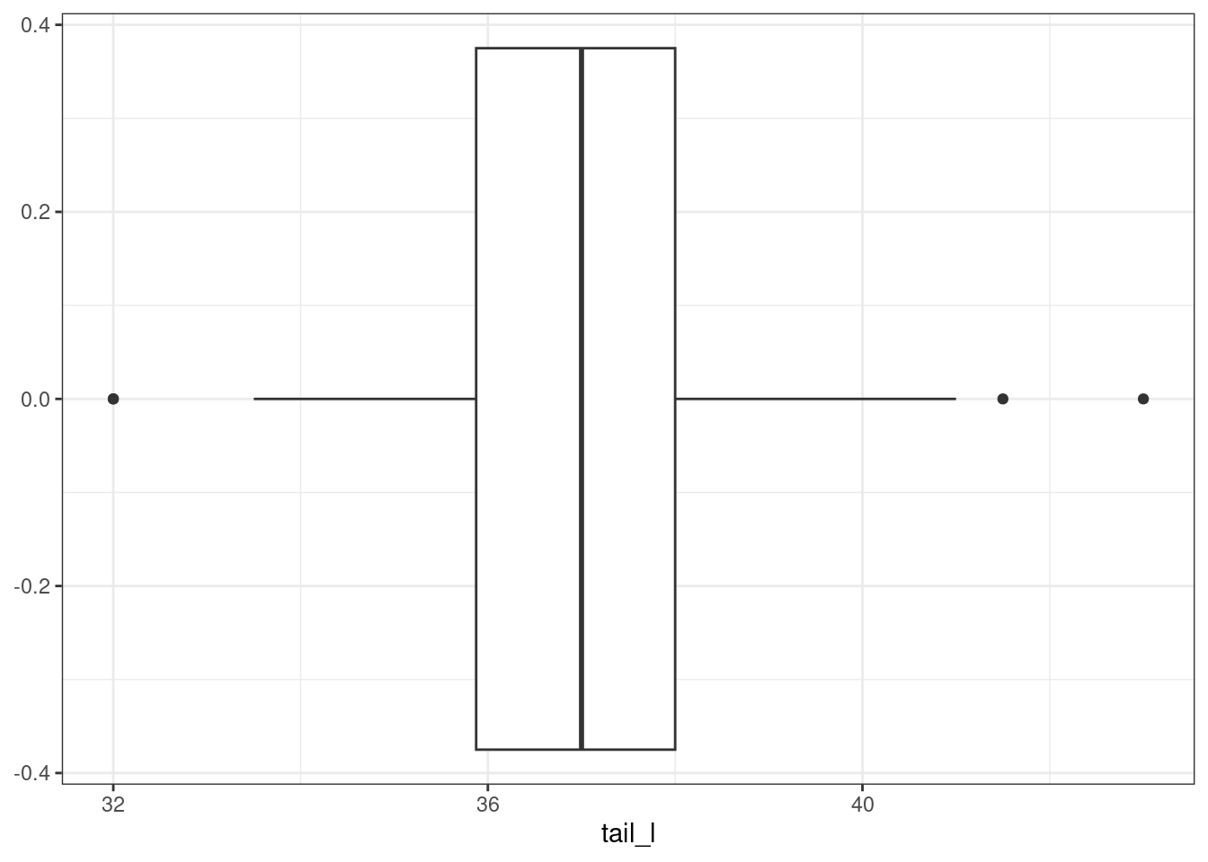
There are some potential outliers for skull width but otherwise not much concern.
pairs(possum[,3:6],lower.panel = panel.smooth)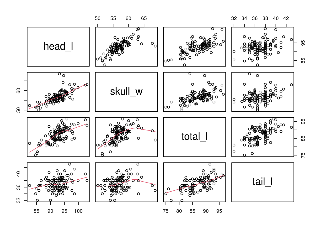 We can see that
 head_l is correlated with the other three variables. This will cause some multicollinearity problems.
- Build a logistic regression model with all the variable. Report a summary of the model.
possum_mod <- glm(pop=="Vic"~.,data=possum,family="binomial")
summary(possum_mod)##
## Call:
## glm(formula = pop == "Vic" ~ ., family = "binomial", data = possum)
##
## Coefficients:
## Estimate Std. Error z value Pr(>|z|)
## (Intercept) 39.2349 11.5368 3.401 0.000672 ***
## sexm -1.2376 0.6662 -1.858 0.063195 .
## head_l -0.1601 0.1386 -1.155 0.248002
## skull_w -0.2012 0.1327 -1.517 0.129380
## total_l 0.6488 0.1531 4.236 2.27e-05 ***
## tail_l -1.8708 0.3741 -5.001 5.71e-07 ***
## ---
## Signif. codes: 0 '***' 0.001 '**' 0.01 '*' 0.05 '.' 0.1 ' ' 1
##
## (Dispersion parameter for binomial family taken to be 1)
##
## Null deviance: 142.787 on 103 degrees of freedom
## Residual deviance: 72.155 on 98 degrees of freedom
## AIC: 84.155
##
## Number of Fisher Scoring iterations: 6
confint(possum_mod)## Waiting for profiling to be done...## 2.5 % 97.5 %
## (Intercept) 18.8530781 64.66444839
## sexm -2.6227018 0.02472167
## head_l -0.4428559 0.10865739
## skull_w -0.4933140 0.04479826
## total_l 0.3768179 0.98455786
## tail_l -2.7170468 -1.23231969- Using the p-values decide if you want to remove a variable(S) and if so build that model.
Let’s remove head_l first.
possum_mod_red <- glm(pop=="Vic"~sex+skull_w+total_l+tail_l,data=possum,family="binomial")
summary(possum_mod_red)##
## Call:
## glm(formula = pop == "Vic" ~ sex + skull_w + total_l + tail_l,
## family = "binomial", data = possum)
##
## Coefficients:
## Estimate Std. Error z value Pr(>|z|)
## (Intercept) 33.5095 9.9053 3.383 0.000717 ***
## sexm -1.4207 0.6457 -2.200 0.027790 *
## skull_w -0.2787 0.1226 -2.273 0.023053 *
## total_l 0.5687 0.1322 4.302 1.69e-05 ***
## tail_l -1.8057 0.3599 -5.016 5.26e-07 ***
## ---
## Signif. codes: 0 '***' 0.001 '**' 0.01 '*' 0.05 '.' 0.1 ' ' 1
##
## (Dispersion parameter for binomial family taken to be 1)
##
## Null deviance: 142.787 on 103 degrees of freedom
## Residual deviance: 73.516 on 99 degrees of freedom
## AIC: 83.516
##
## Number of Fisher Scoring iterations: 6Since head_l was correlated with the other variables, removing it has increased the precision, decreased the standard error, of the other predictors. There p-values are all now less than 0.05.
- For any variable you decide to remove, build a 95% confidence interval for the parameter.
confint(possum_mod)## Waiting for profiling to be done...## 2.5 % 97.5 %
## (Intercept) 18.8530781 64.66444839
## sexm -2.6227018 0.02472167
## head_l -0.4428559 0.10865739
## skull_w -0.4933140 0.04479826
## total_l 0.3768179 0.98455786
## tail_l -2.7170468 -1.23231969We are 95% confident that the true slope coefficient for head_l is between -0.44 and 0.108.
The bootstrap is not working for this problem. It may be that we have convergence issues when we resample the data. This is a reminder that we need to be careful and not just run methods without checking results. Here is the code:
head(results[,1:5])## Intercept sexm head_l skull_w total_l
## 1 -1184.61875 2.122389e+01 3.861561e+00 2.749263e+00 7.274005e+00
## 2 6371.55550 -1.301514e+02 1.023732e+01 -2.738816e+01 -1.076913e+01
## 3 -9612.61941 -2.392900e+03 -1.875252e+02 5.782027e+02 -2.820691e+02
## 4 -25.18662 -1.852185e+01 2.097593e+01 -1.353619e+01 1.483815e+01
## 5 -26.56607 -1.398995e-14 -2.258909e-14 6.528545e-15 2.388756e-14
## 6 -1025.00035 6.159665e+01 2.526181e+01 -2.032143e+01 1.438639e+01
results %>%
  gf_histogram(~head_l,fill="cyan",color = "black") %>%
  gf_theme(theme_bw()) %>%
  gf_labs(title="Bootstrap sampling distribtuion",
          x="sex paramater estimate")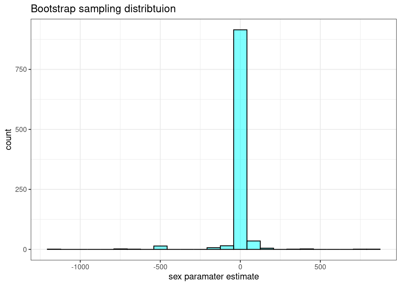
cdata(~head_l,data=results)## lower upper central.p
## 2.5% -122.7029 63.61867 0.95This interval is too large. The resampling process has too much variation in it. This could be due to the small sample size and the multicollinearity.
- Explain why the remaining parameter estimates change between the two models.
When coefficient estimates are sensitive to which variables are included in the model, this typically indicates that some variables are collinear. For example, a possum’s gender may be related to its head length, which would explain why the coefficient (and p-value) for sex male changed when we removed the head length variable. Likewise, a possum’s skull width is likely to be related to its head length, probably even much more closely related than the head length was to gender.
- Write out the form of the model. Also identify which of the following variables are positively associated (when controlling for other variables) with a possum being from Victoria:
head_l,skull_w,total_l, andtail_l.
We dropped head_l from the model. Here is the equation:
\[ \log_{e}\left( \frac{p_i}{1-p_i} \right) = 33.5 - 1.42 \text{ sex} -0.28 \text{ skull width} + 0.57 \text{ total length} - 1.81 \text{ tail length} \]
Only total_l is positively association with the probability of being from Victoria.
- Suppose we see a brushtail possum at a zoo in the US, and a sign says the possum had been captured in the wild in Australia, but it doesn’t say which part of Australia. However, the sign does indicate that the possum is male, its skull is about 63 mm wide, its tail is 37 cm long, and its total length is 83 cm. What is the reduced model’s computed probability that this possum is from Victoria? How confident are you in the model’s accuracy of this probability calculation?
Let’s predict the outcome. We use response for the type to put the answer in the form of a probability. See the help menu on predict.glm for more information.
predict(possum_mod_red,newdata = data.frame(sex="m",skull_w=63,tail_l=37,total_l=83),
        type="response",se.fit = TRUE)
## $fit
## 1
## 0.006205055
##
## $se.fit
## 1
## 0.008011468
##
## $residual.scale
## [1] 1While the probability, 0.006, is very near zero, we have not run diagnostics on the model. We should also have a little skepticism that the model will hold for a possum found in a US zoo. However, it is encouraging that the possum was caught in the wild.
As a rough sense of the accuracy, we will use the standard error. The errors are really binomial but we are trying to use a normal approximation. If you remember back to our block on probability, with such a low probability, this assumption of normality is suspect. However, we will use it to give us an upper bound.
0.0062+c(-1,1)*1.96*.008## [1] -0.00948 0.02188So at most, the probability of the possum being from Victoria is 2%.
32.2.2 Problem 2
Medical school admission
The file MedGPA.csv in the data folder has information on medical school admission status and GPA and standardized test scores gathered on 55 medical school applicants from a liberal arts college in the Midwest.
The variables are:
Accept Status: A=accepted to medical school or D=denied admission
Acceptance: Indicator for Accept: 1=accepted or 0=deniedSex: F=female or M=maleBCPM: Bio/Chem/Physics/Math grade point averageGPA: College grade point averageVR: Verbal reasoning (subscore)PS: Physical sciences (subscore)WS: Writing sample (subcore)BS: Biological sciences (subscore)MCAT: Score on the MCAT exam (sum of CR+PS+WS+BS)Apps: Number of medical schools applied to
- Build a logistic regression model to predict
AcceptancefromGPAand `Sex.
MedGPA <- read_csv("data/MedGPA.csv")
glimpse(MedGPA)## Rows: 55
## Columns: 11
## $ Accept <chr> "D", "A", "A", "A", "A", "A", "A", "D", "A", "A", "A", "A",…
## $ Acceptance <dbl> 0, 1, 1, 1, 1, 1, 1, 0, 1, 1, 1, 1, 1, 0, 0, 1, 0, 1, 0, 1,…
## $ Sex <chr> "F", "M", "F", "F", "F", "M", "M", "M", "F", "F", "F", "F",…
## $ BCPM <dbl> 3.59, 3.75, 3.24, 3.74, 3.53, 3.59, 3.85, 3.26, 3.74, 3.86,…
## $ GPA <dbl> 3.62, 3.84, 3.23, 3.69, 3.38, 3.72, 3.89, 3.34, 3.71, 3.89,…
## $ VR <dbl> 11, 12, 9, 12, 9, 10, 11, 11, 8, 9, 11, 11, 8, 9, 11, 12, 8…
## $ PS <dbl> 9, 13, 10, 11, 11, 9, 12, 11, 10, 9, 9, 8, 10, 9, 8, 8, 8, …
## $ WS <dbl> 9, 8, 5, 7, 4, 7, 6, 8, 6, 6, 8, 4, 7, 4, 6, 8, 8, 9, 5, 8,…
## $ BS <dbl> 9, 12, 9, 10, 11, 10, 11, 9, 11, 10, 11, 8, 10, 10, 7, 10, …
## $ MCAT <dbl> 38, 45, 33, 40, 35, 36, 40, 39, 35, 34, 39, 31, 35, 32, 32,…
## $ Apps <dbl> 5, 3, 19, 5, 11, 5, 5, 7, 5, 11, 6, 9, 5, 8, 15, 6, 6, 1, 5…
med_mod<-glm(Accept=="D"~GPA+Sex,data=MedGPA,family=binomial)
summary(med_mod)##
## Call:
## glm(formula = Accept == "D" ~ GPA + Sex, family = binomial, data = MedGPA)
##
## Coefficients:
## Estimate Std. Error z value Pr(>|z|)
## (Intercept) 21.0680 6.4025 3.291 0.001000 ***
## GPA -6.1324 1.8283 -3.354 0.000796 ***
## SexM 1.1697 0.7178 1.629 0.103210
## ---
## Signif. codes: 0 '***' 0.001 '**' 0.01 '*' 0.05 '.' 0.1 ' ' 1
##
## (Dispersion parameter for binomial family taken to be 1)
##
## Null deviance: 75.791 on 54 degrees of freedom
## Residual deviance: 53.945 on 52 degrees of freedom
## AIC: 59.945
##
## Number of Fisher Scoring iterations: 5- Generate a 95% confidence interval for the coefficient associated with
GPA.
confint(med_mod)## Waiting for profiling to be done...## 2.5 % 97.5 %
## (Intercept) 10.0651173 35.579760
## GPA -10.2977983 -3.007544
## SexM -0.1720454 2.697436Let’s try the bootstrap for this problem.
set.seed(819)
results_med <- do(1000)*glm(Accept=="D"~GPA+Sex,data=resample(MedGPA),family=binomial)
## Warning: glm.fit: fitted probabilities numerically 0 or 1 occurred
results_med %>%
  gf_histogram(~GPA,fill="cyan",color = "black") %>%
  gf_theme(theme_bw()) %>%
  gf_labs(title="Bootstrap sampling distribtuion",
          x="GPA paramater estimate")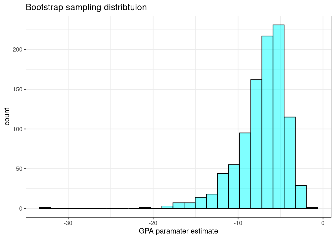
cdata(~GPA,data=results_med)## lower upper central.p
## 2.5% -14.2047 -3.213036 0.95This is not so bad. It appears that the distribution of GPA is skewed to the left.
- Fit a model with a polynomial of degree 2 in the
GPA. DropSexfrom the model. Does a quadratic fit improve the model?
summary(med_mod2)##
## Call:
## glm(formula = Accept == "D" ~ poly(GPA, 2), family = binomial,
## data = MedGPA)
##
## Coefficients:
## Estimate Std. Error z value Pr(>|z|)
## (Intercept) -0.3301 0.3582 -0.921 0.356822
## poly(GPA, 2)1 -10.7293 3.0664 -3.499 0.000467 ***
## poly(GPA, 2)2 -3.4967 3.0987 -1.128 0.259133
## ---
## Signif. codes: 0 '***' 0.001 '**' 0.01 '*' 0.05 '.' 0.1 ' ' 1
##
## (Dispersion parameter for binomial family taken to be 1)
##
## Null deviance: 75.791 on 54 degrees of freedom
## Residual deviance: 55.800 on 52 degrees of freedom
## AIC: 61.8
##
## Number of Fisher Scoring iterations: 4The quadratic term did not improve the model.
- Fit a model with just
GPAand interpret the coefficient.
## # A tibble: 2 × 5
##   term        estimate std.error statistic  p.value
##   <chr>          <dbl>     <dbl>     <dbl>    <dbl>
## 1 (Intercept)    19.2       5.63      3.41 0.000644
## 2 GPA            -5.45      1.58     -3.45 0.000553
exp(-5.454166)## [1] 0.004278444An increase of 1 in a student’s GPA decreases the odds of being denied acceptance by 0.00428. Remember that this is not a probability. As a reminder an odds of \(\frac{1}{2}\) means the probability of success is \(\frac{1}{3}\). An odds of 1 means a probability of success of \(\frac{1}{2}\). Assume the initial odds are 1 if the odds are now 0.00428 smaller, then the probability of success is \(\frac{428}{10428}\) or 0.04. The probability decreased by an order of magnitude.
- Try to add different predictors to come up with your best model. Do not use Acceptance and MCAT in the model.
tidy(glm(Accept=="D"~.-Acceptance-MCAT,data=MedGPA,family=binomial)) %>%
  mutate(p.adj=p.adjust(p.value)) %>%
  select(term,p.value,p.adj)
## # A tibble: 9 × 3
## term p.value p.adj
## <chr> <dbl> <dbl>
## 1 (Intercept) 0.00279 0.0251
## 2 SexM 0.110 0.551
## 3 BCPM 0.376 1
## 4 GPA 0.150 0.600
## 5 VR 0.799 1
## 6 PS 0.0305 0.213
## 7 WS 0.0491 0.295
## 8 BS 0.00490 0.0392
## 9 Apps 0.728 1Let’s take out VR.
tidy(glm(Accept=="D"~.-Acceptance-MCAT-VR,data=MedGPA,family=binomial)) %>%
  mutate(p.adj=p.adjust(p.value)) %>%
  select(term,p.value,p.adj)
## # A tibble: 8 × 3
## term p.value p.adj
## <chr> <dbl> <dbl>
## 1 (Intercept) 0.00239 0.0191
## 2 SexM 0.0681 0.272
## 3 BCPM 0.362 0.723
## 4 GPA 0.143 0.430
## 5 PS 0.0280 0.168
## 6 WS 0.0452 0.226
## 7 BS 0.00476 0.0333
## 8 Apps 0.742 0.742Now let’s take out Apps.
tidy(glm(Accept=="D"~.-Acceptance-MCAT-VR-Apps,data=MedGPA,family=binomial)) %>%
  mutate(p.adj=p.adjust(p.value)) %>%
  select(term,p.value,p.adj)
## # A tibble: 7 × 3
## term p.value p.adj
## <chr> <dbl> <dbl>
## 1 (Intercept) 0.00147 0.0103
## 2 SexM 0.0272 0.133
## 3 BCPM 0.379 0.379
## 4 GPA 0.120 0.240
## 5 PS 0.0266 0.133
## 6 WS 0.0385 0.133
## 7 BS 0.00477 0.0286Next, let’s remove BCPM.
tidy(glm(Accept=="D"~.-Acceptance-MCAT-VR-Apps-BCPM,
         data=MedGPA,family=binomial)) %>%
  mutate(p.adj=p.adjust(p.value)) %>%
  select(term,p.value,p.adj)
## # A tibble: 6 × 3
## term p.value p.adj
## <chr> <dbl> <dbl>
## 1 (Intercept) 0.00123 0.00739
## 2 SexM 0.0142 0.0567
## 3 GPA 0.0315 0.0901
## 4 PS 0.0300 0.0901
## 5 WS 0.0401 0.0901
## 6 BS 0.00537 0.0269Now WS.
tidy(glm(Accept=="D"~.-Acceptance-MCAT-VR-Apps-BCPM-WS,
         data=MedGPA,family=binomial)) %>%
  mutate(p.adj=p.adjust(p.value)) %>%
  select(term,p.value,p.adj)
## # A tibble: 5 × 3
## term p.value p.adj
## <chr> <dbl> <dbl>
## 1 (Intercept) 0.000584 0.00292
## 2 SexM 0.0168 0.0504
## 3 GPA 0.0366 0.0732
## 4 PS 0.0634 0.0732
## 5 BS 0.0100 0.0401Maybe PS.
tidy(glm(Accept=="D"~.-Acceptance-MCAT-VR-Apps-BCPM-WS-PS,
         data=MedGPA,family=binomial)) %>%
  mutate(p.adj=p.adjust(p.value)) %>%
  select(term,p.value,p.adj)
## # A tibble: 4 × 3
## term p.value p.adj
## <chr> <dbl> <dbl>
## 1 (Intercept) 0.000574 0.00230
## 2 SexM 0.0306 0.0611
## 3 GPA 0.0325 0.0611
## 4 BS 0.00448 0.0134We will stop there. There has to be a better way. Machine learning and advanced regression courses explore how to select predictors and improve a model.
- Generate a confusion matrix for the best model you have developed.
med_mod2<-glm(Accept=="D"~Sex+GPA+BS,
         data=MedGPA,family=binomial)
summary(med_mod2)##
## Call:
## glm(formula = Accept == "D" ~ Sex + GPA + BS, family = binomial,
## data = MedGPA)
##
## Coefficients:
## Estimate Std. Error z value Pr(>|z|)
## (Intercept) 27.4608 7.9721 3.445 0.000572 ***
## SexM 1.9885 0.9193 2.163 0.030543 *
## GPA -4.2900 2.0062 -2.138 0.032484 *
## BS -1.3752 0.4838 -2.843 0.004471 **
## ---
## Signif. codes: 0 '***' 0.001 '**' 0.01 '*' 0.05 '.' 0.1 ' ' 1
##
## (Dispersion parameter for binomial family taken to be 1)
##
## Null deviance: 75.791 on 54 degrees of freedom
## Residual deviance: 40.835 on 51 degrees of freedom
## AIC: 48.835
##
## Number of Fisher Scoring iterations: 6
augment(med_mod2,type.predict = "response") %>%
  rename(actual=starts_with('Accept ==')) %>%
  transmute(result=as.integer(.fitted>0.5),
            actual=as.integer(actual)) %>%
  table()
## actual
## result 0 1
## 0 26 4
## 1 4 21This model has an accuracy of \(\frac{47}{55}\) or 85.5%.
- Find a 95% confidence interval for the probability a female student with a 3.5 GPA, a
BCPMof 3.8, a verbal reasoning score of 10, a physical sciences score of 9, a writing sample score of 8, a biological score of 10, a MCAT score of 40, and who applied to 5 medical schools.
predict(med_mod2,newdata = data.frame(Sex="F",
                                      GPA=3.5,
                                      BS=10),
        type="response",se.fit = TRUE)
## $fit
## 1
## 0.2130332
##
## $se.fit
## 1
## 0.1122277
##
## $residual.scale
## [1] 1
0.2130332+c(-1,1)*1.96*.1122277## [1] -0.006933092 0.432999492For a female students with a GPA of 3.5 and a biological score of 10, we are 95% confident that the probability of being denied acceptance to medical school is between 0 and .433.
Let’s try a bootstrap.
set.seed(729)
results <- do(1000)*glm(Accept=="D"~Sex+GPA+BS,
                      data=resample(MedGPA),
                      family=binomial)
head(results)## Intercept SexM GPA BS .row .index
## 1 204.23984 20.701630 -4.547781 -20.801516 1 1
## 2 16.78193 1.373795 -2.508340 -0.908112 1 2
## 3 36.09536 4.170571 -7.479463 -1.219088 1 3
## 4 1104.42269 105.236280 -90.461857 -86.132398 1 4
## 5 25.37989 1.139262 -3.729948 -1.331750 1 5
## 6 26.58307 3.197072 -3.426165 -1.772581 1 6
cdata(~pred,data=results_pred)## lower upper central.p
## 2.5% 7.77316e-10 0.5032905 0.95This is close to what we found and does not make the assumption the probability of success is normally distributed.