11 Continuous Random Variables

11.1 Objectives

1. Define and properly use in context all new terminology, to include: probability density function (pdf) and cumulative distribution function (cdf) for continuous random variables.

2. Given a continuous random variable, find probabilities using the pdf and/or the cdf.

3. Find the mean and variance of a continuous random variable.

11.2 Homework

11.2.1 Problem 1

Let $X$ be a continuous random variable on the domain $-k \leq X \leq k$. Also, let $f(x)=\frac{x^2}{18}$.

1. Assume that $f(x)$ is a valid pdf. Find the value of $k$.

Because $f$ is a valid pdf, we know that $\int_{-k}^k \frac{x^2}{18}\mathop{}\!\mathrm{d}x = 1$. So, $$\int_{-k}^k \frac{x^2}{18}\mathop{}\!\mathrm{d}x = \frac{x^3}{54}\bigg|_{-k}^k = \frac{k^3}{54}-\frac{-k^3}{54}=\frac{k^3}{27}=1$$

Thus, $k=3$.

Using R, see if you can follow the code.

my_pdf <- function(x)integrate(function(y)y^2/18,-x,x)$value

my_pdf<-Vectorize(my_pdf)

domain <- seq(.01,5,.1)
gf_line(my_pdf(domain)~domain) %>%
  gf_theme(theme_classic()) %>%
  gf_labs(title="Cumulative probability for different values of k",x="k",y="Cummulative Probability") %>%
  gf_hline(yintercept = 1,color = "blue")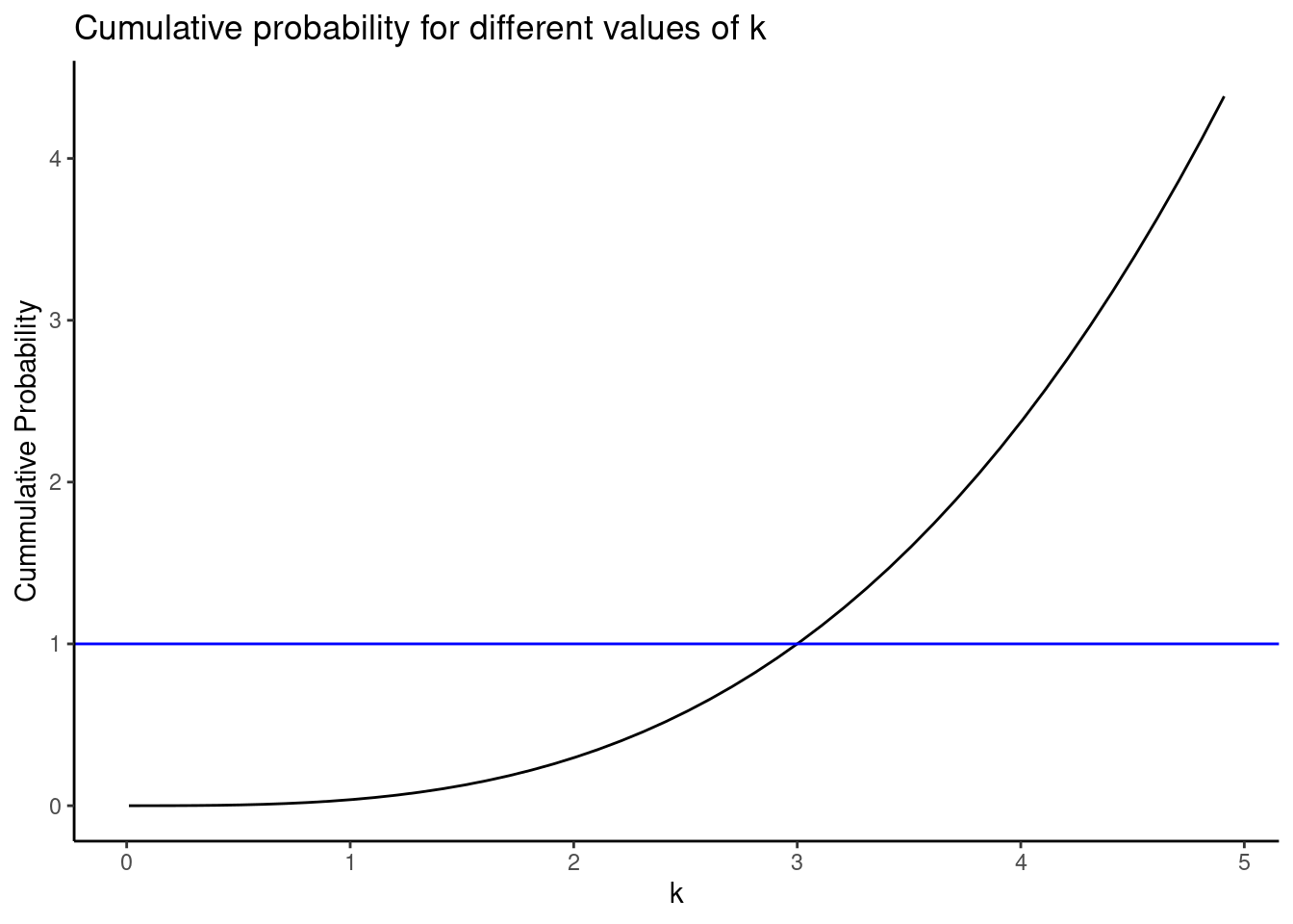

Looks like $k \approx 3$ from the plot.

uniroot(function(x)my_pdf(x)-1,c(-10,10))$root

## [1] 2.999997

2. Plot the pdf of $X$.

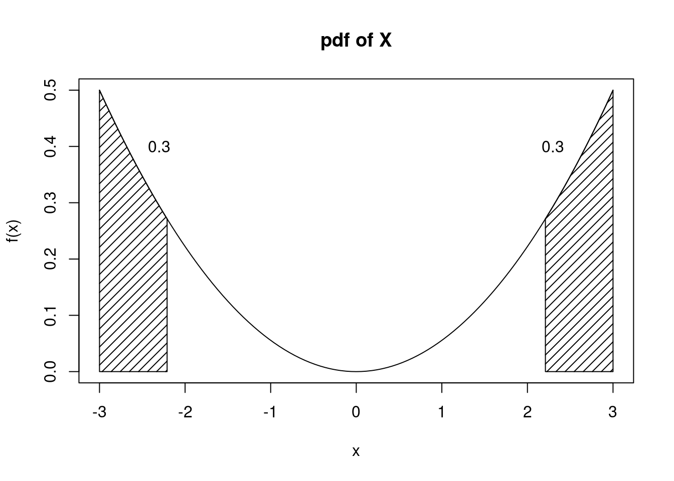
x<-seq(-3,3,0.001)
fx<-x^2/18
gf_line(fx~x,ylab="f(x)",title="pdf of X") %>%
  gf_theme(theme_classic())

ggplot(data.frame(x=c(-3, 3)), aes(x)) + 
 stat_function(fun=function(x) x^2/18) +
  theme_classic() +
  labs(y="f(x)",title="pdf of X")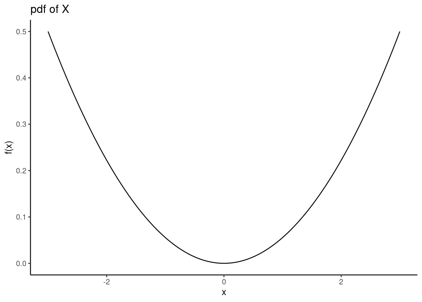

curve(x^2/18,from=-3,to=3,ylab="f(x)",main="pdf of X")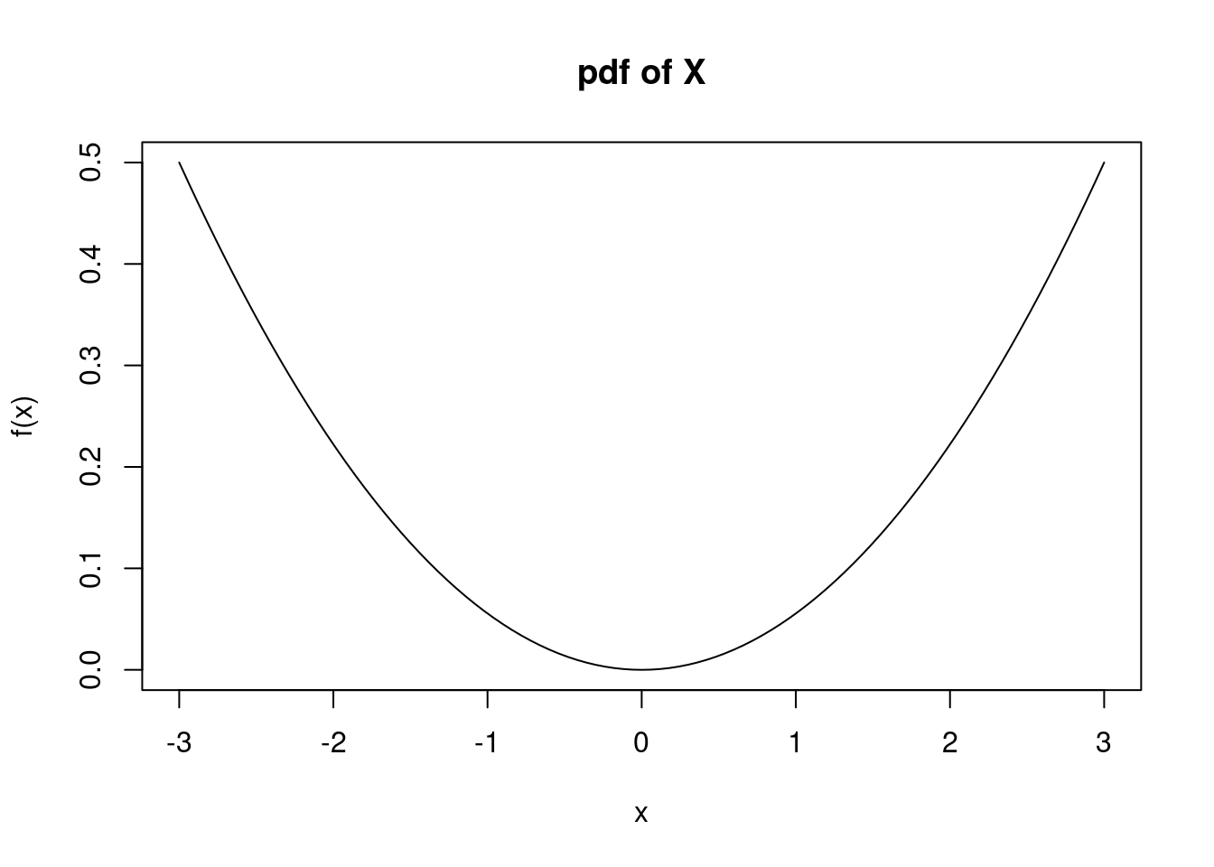

3. Find and plot the cdf of $X$. $$F_X(x)=\mbox{P}(X\leq x)=\int_{-3}^x \frac{t^2}{18}\mathop{}\!\mathrm{d}t = \frac{t^3}{54}\bigg|_{-3}^x = \frac{x^3}{54}+\frac{1}{2}$$

$$F_X(x)=\left\{\begin{array}{ll} 0, & x<-3 \\ \frac{x^3}{54}+\frac{1}{2}, & -3\leq x \leq 3 \\ 1, & x>3 \end{array}\right.$$

x<-seq(-3.5,3.5,0.001)
fx<-pmin(1,(1*(x>=-3)*(x^3/54+1/2)))
gf_line(fx~x,ylab="F(x)",title="cdf of X") %>%
  gf_theme(theme_classic())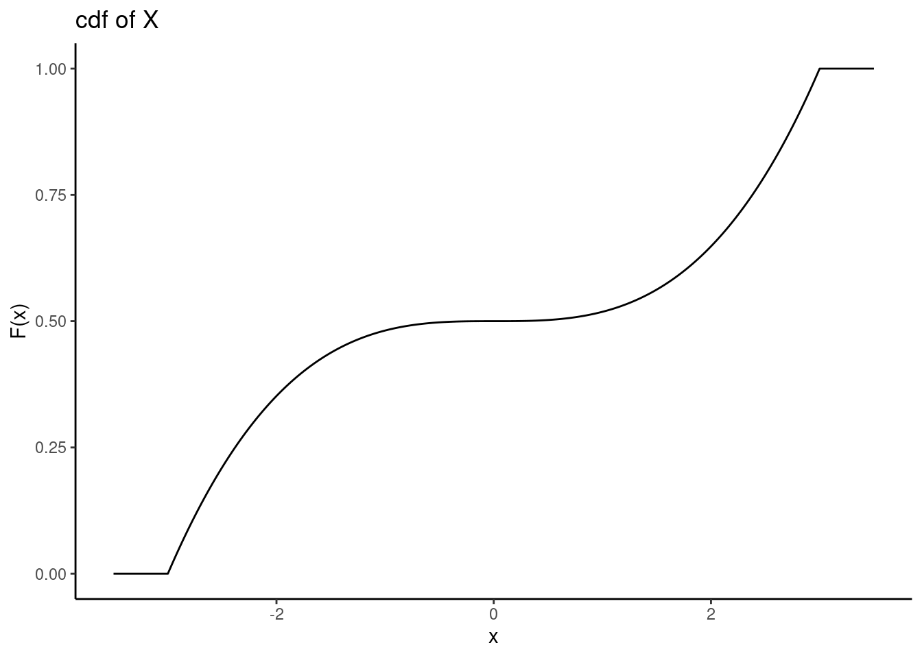

4. Find $\mbox{P}(X<1)$. $$\mbox{P}(X<1)=F(1)=\frac{1}{54}+\frac{1}{2}=0.519$$

integrate(function(x)x^2/18,-3,1)

## 0.5185185 with absolute error < 5.8e-15

5. Find $\mbox{P}(1.5<X\leq 2.5)$. $$\mbox{P}(1.5< X \leq 2.5)=F(2.5)-F(1.5)=\frac{2.5^3}{54}+\frac{1}{2}-\frac{1.5^3}{54}-\frac{1}{2}=0.227$$

integrate(function(x)x^2/18,1.5,2.5)

## 0.2268519 with absolute error < 2.5e-15

6. Find the 80th percentile of $X$ (the value $x$ for which 80% of the distribution is to the left of that value).

Need $x$ such that $F(x)=0.8$. Solving $\frac{x^3}{54}+\frac{1}{2}=0.8$ for $x$ yields $x=2.530$.

uniroot(function(x)x^3/54+.5-.8,c(-3,3))

## $root
## [1] 2.530293
## 
## $f.root
## [1] -1.854422e-06
## 
## $iter
## [1] 6
## 
## $init.it
## [1] NA
## 
## $estim.prec
## [1] 6.103516e-05

7. Find the value $x$ such that $\mbox{P}(-x \leq X \leq x)=0.4$.

Because this distribution is symmetric, finding $x$ is equivalent to finding $x$ such that $\mbox{P}(X>x)=0.3$. (It helps to draw a picture). Thus, we need $x$ such that $F(x)=0.7$. Solving $\frac{x^3}{54}+\frac{1}{2}=0.7$ for $x$ yields $x=2.210$.

8. Find the mean and variance of $X$. $$\mbox{E}(X)=\int_{-3}^3 x\cdot\frac{x^2}{18}\mathop{}\!\mathrm{d}x = \frac{x^4}{72}\bigg|_{-3}^3=\frac{81}{72}-\frac{81}{72} = 0$$

$$\mbox{E}(X^2)=\int_{-3}^3 x^2\cdot\frac{x^2}{18}\mathop{}\!\mathrm{d}x = \frac{x^5}{90}\bigg|_{-3}^3=\frac{243}{90}-\frac{-243}{90} = 5.4$$

$$\mbox{Var}(X)=\mbox{E}(X^2)-\mbox{E}(X)^2=5.4-0^2=5.4$$

1. Simulate 10000 values from this distribution and plot the density.

This is tricky since we need a cube root function. Just raising to the one-third power won’t work. Let’s write our own function.

cuberoot <- function(x) {
  sign(x) * abs(x)^(1/3)}

set.seed(4)
results <- do(10000)*cuberoot((runif(1)-.5)*54)

results %>%
  gf_dens(~cuberoot) %>%
  gf_theme(theme_classic()) %>%
  gf_labs(title="pdf from simulation",x="x",y="f(x)")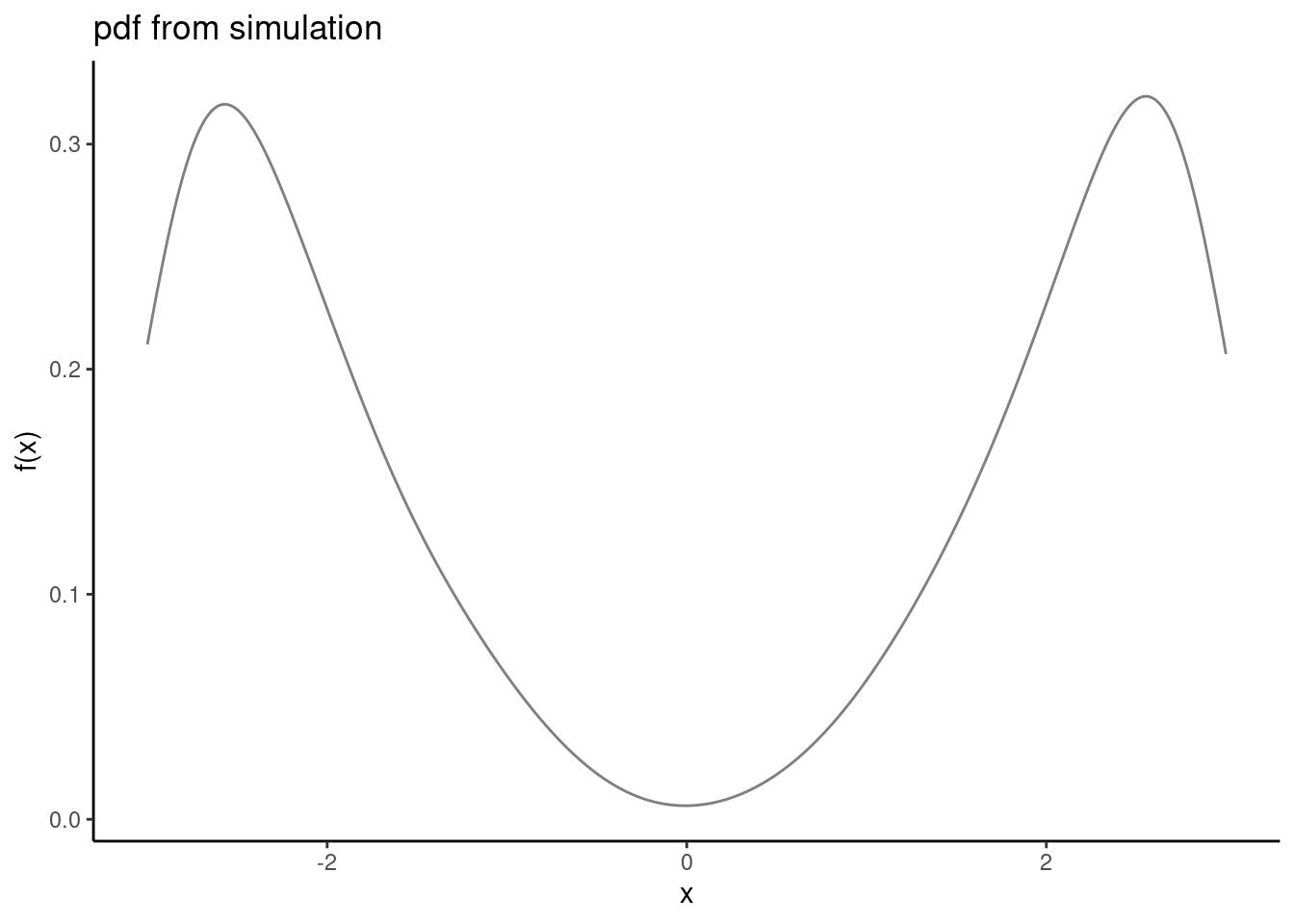 

Notice that the smoothing operation goes past the support of $X$ and thus shows a concave down curve. We could clean up by limiting the x-axis to the interval [-3,3].

inspect(results)

## 
## quantitative variables:  
##       name   class       min        Q1     median       Q3      max
## 1 cuberoot numeric -2.999981 -2.382864 -0.1574198 2.376346 2.999347
##           mean       sd     n missing
## 1 -0.002416475 2.322639 10000       0

11.2.2 Problem 2

Let $X$ be a continuous random variable. Prove that the cdf of $X$, $F_X(x)$ is a non-decreasing function. (Hint: show that for any $a < b$, $F_X(a) \leq F_X(b)$.)

Let $a<b$, where $a$ and $b$ are both in the domain of $X$. Note that $F_X(a)=\mbox{P}(X\leq a)$ and $F_X(b)=\mbox{P}(X\leq b)$. Since $a<b$, we can partition $\mbox{P}(X\leq b)$ as $\mbox{P}(X\leq a)+\mbox{P}(a < X \leq b)$. One of the axioms of probability is that a probability must be non-negative, so I know that $\mbox{P}(a < X \leq b)\geq 0$. Thus, $$\mbox{P}(X\leq b)=\mbox{P}(X\leq a)+\mbox{P}(a < X \leq b) \geq \mbox{P}(X\leq a)$$

So, we have shown that $F_X(a)\leq F_X(b)$. Thus, $F_X(x)$ is a non-decreasing function.

Textbook