13 Named Continuous Distributions
13.1 Objectives
Recognize when to use common continuous distributions (Uniform, Exponential, Gamma, Normal, Weibull, and Beta), identify parameters, and find moments.
Use
Rto calculate probabilities and quantiles involving random variables with common continuous distributions.Understand the relationship between the Poisson process and the Poisson & Exponential distributions.
Know when to apply and then use the memory-less property.
13.2 Homework
For problems 1-3 below, 1) define a random variable that will help you answer the question, 2) state the distribution and parameters of that random variable; 3) determine the expected value and variance of that random variable, and 4) use that random variable to answer the question.
13.2.1 Problem 1
On a given Saturday, suppose vehicles arrive at the USAFA North Gate according to a Poisson process at a rate of 40 arrivals per hour.
- Find the probability no vehicles arrive in 10 minutes.
\(X\): number of vehicles that arrive in 10 minutes
\(X\sim \textsf{Pois}(\lambda=40/6=6.67)\) and \(\mbox{E}(X)=\mbox{Var}(X)=6.67\).
\(\mbox{P}(\mbox{no arrivals in 10 minutes})=\mbox{P}(X=0)=\frac{6.67^0 e^{-6.67}}{0!}=e^{-6.67}\)
exp(-40/6)## [1] 0.001272634
##or
dpois(0,40/6)
## [1] 0.001272634or, using the exponential distribution:
\(Y\): time in minutes until the next arrival
\(Y\sim \textsf{Expon}(\lambda=40/60=0.667)\) and \(\mbox{E}(Y)=1.5\) and \(\mbox{Var}(Y)=2.25\).
\[ \mbox{P}(\mbox{at least 10 minutes until the next arrival})=\mbox{P}(Y\geq 10)=\int_{10}^\infty \frac{2}{3}e^{-\frac{2}{3}y}\mathop{}\!\mathrm{d}y \]
1-pexp(10,2/3)## [1] 0.001272634or using simulation:
## [1] 0.00126
mean(rexp(100000,2/3) >=10)## [1] 0.00127- Find the probability that at least 5 minutes will pass before the next arrival.
\(Y\): same as in part a
\[ \mbox{P}(\mbox{at least 5 minutes until next arrival})=\mbox{P}(Y\geq 5)=\int_{5}^\infty \frac{2}{3}e^{-\frac{2}{3}y}\mathop{}\!\mathrm{d}y \]
1-pexp(5,2/3)## [1] 0.03567399- Find the probability that the next vehicle will arrive between 2 and 10 minutes from now.
Same \(Y\) as defined above.
## [1] 0.2623245- Find the probability that at least 7 minutes will pass before the next arrival, given that 2 minutes have already passed. Compare this answer to part (b). This is an example of the memoryless property of the exponential distribution. \[ \mbox{P}(Y\geq 7|Y\geq 2) = \frac{\mbox{P}(Y\geq 7, Y\geq 2)}{\mbox{P}(Y\geq 2)} = \frac{\mbox{P}(Y\geq 7)}{\mbox{P}(Y\geq 2)} \]
## [1] 0.03567399This is the same answer and a result of the memoryless property.
- Fill in the blank. There is a probability of 90% that the next vehicle will arrive within __ minutes. This value is known as the 90% percentile of the random variable.
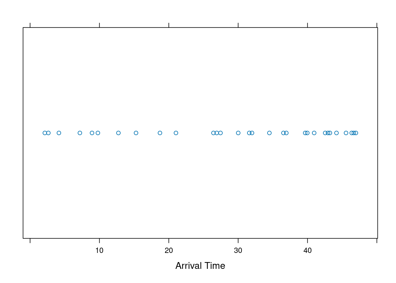
qexp(0.9,2/3)## [1] 3.453878- Use the function
stripplot()to visualize the arrival of 30 vehicles using a random sample from the appropriate exponential distribution.
13.2.2 Problem 2
Suppose time until computer errors on the F-35 follows a Gamma distribution with mean 20 hours and variance 10.
- Find the probability that 20 hours pass without a computer error.
\(X\): time in hours until next computer error.
\(X\sim \textsf{Gamma}(\alpha = 40, \lambda = 2)\)
We need to find \(\alpha\) and \(\lambda\) from the given moments.
\(\mbox{E}(X) = 20 = \frac{\alpha}{\lambda}\)
\(\mbox{Var}(X) = 10 = \frac{\alpha}{\lambda^2}\)
Notice that \(\frac{\mbox{E}(X)}{\mbox{Var}(X)} = \lambda = \frac{20}{10}=2\) and then using \(\mbox{E}(X) = 20 = \frac{\alpha}{\lambda}\) we get \(\alpha = 40\).
\(\mbox{P}(X\geq 20)\):
1-pgamma(20,shape=40,rate=2)## [1] 0.4789711- Find the probability that 45 hours pass without a computer error, given that 25 hours have already passed. Does the memoryless property apply to the Gamma distribution? \[ P(X\geq 45|X\geq 25) = \frac{P(X\geq 45, X\geq 25)}{P(X\geq 25)} = \frac{P(X\geq 45)}{P(X\geq 25)} \]
## [1] 1.77803e-08No, the memoryless property does not apply to the Gamma distribution.
- Find \(a\) and \(b\) where there is a 95% probability that the time until next computer error will be between \(a\) and \(b\). (Note: technically, there are many answers to this question, but find \(a\) and \(b\) such that each tail has equal probability.)
## [1] 14.28829 26.65714So, there is a 95% probability that the time until next computer error will be in the time interval \([14.29, 26.66]\). This uses the central 95% of the gamma distribution.
qgamma(0.95, 40, 2)## [1] 25.46987Another answer is between \([0, 25.47]\). This uses the lower 95% of the gamma distribution.
13.2.3 Problem 3
Suppose PFT scores in the cadet wing follow a normal distribution with mean 330 and standard deviation 50.
- Find the probability a randomly selected cadet has a PFT score higher than 450.
\(X\): PFT score of a randomly selected cadet
\(X\sim \textsf{Norm}(\mu=330,\sigma=50)\)
\(\mbox{E}(X) = 330\) and \(\mbox{Var}(X)=50^2=2500\).
1-pnorm(450,330,50)## [1] 0.008197536- Find the probability a randomly selected cadet has a PFT score within 2 standard deviations of the mean.
Need \(\mbox{P}(230 \leq X \leq 430)\).
## [1] 0.9544997- Find \(a\) and \(b\) such that 90% of PFT scores will be between \(a\) and \(b\).
Need \(a\) such that \(\mbox{P}(X\leq a)=0.05\) and \(b\) such that \(\mbox{P}(X\geq b)=0.05\):
qnorm(0.05,330,50)## [1] 247.7573
qnorm(0.95,330,50)## [1] 412.2427- Find the probability a randomly selected cadet has a PFT score higher than 450 given he/she is among the top 10% of cadets.
Need \(\mbox{P}(X>450|X>x_{0.9})\) where \(x_{0.9}\) is the 90th percentile of \(X\).
The 90th percentile is:
qnorm(0.9,330,50)## [1] 394.0776\[ \mbox{P}(X>450|X>x_{0.9})=\frac{\mbox{P}(X>450, X>x_{0.9})}{\mbox{P}(X>x_{0.9})}=\frac{\mbox{P}(X>450, X>394.08)}{\mbox{P}(X>x_{0.9})}=\frac{\mbox{P}(X>450)}{0.1} \]
This is assuming that \(x_{0.9}<450\). Otherwise the problem is trivial and the probability is 1.
(1-pnorm(450,330,50))/0.1## [1] 0.0819753613.2.4 Problem 4
Let \(X \sim \textsf{Beta}(\alpha=1,\beta=1)\). Show that \(X\sim \textsf{Unif}(0,1)\). Hint: write out the beta distribution pdf where \(\alpha=1\) and \(\beta=1\).
The beta pdf is: \[ f_X(x)=\frac{\Gamma(\alpha + \beta)}{\Gamma(\alpha)\Gamma(\beta)}x^{\alpha-1}(1-x)^{\beta-1} \]
When \(X\sim\textsf{Beta}(\alpha=1,\beta=1)\), this becomes: \[ f_X(x)=\frac{\Gamma(2)}{\Gamma(1)\Gamma(1)}x^{1-1}(1-x)^{1-1} = 1 \]
13.2.5 Problem 5
When using R to calculate probabilities related to the gamma distribution, we often use pgamma. Recall that pgamma is equivalent to the cdf of the gamma distribution. If \(X\sim\textsf{Gamma}(\alpha,\lambda)\), then
\[
\mbox{P}(X\leq x)=\textsf{pgamma(x,alpha,lambda)}
\]
The dgamma function exists in R too. In plain language, explain what dgamma returns. I’m not looking for the definition found in R documentation. I’m looking for a simple description of what that function returns. Is the output of dgamma useful? If so, how?
The dgamma function returns the value of probability density function. While this is not a probability, it is still a useful quantity. It can be said that larger densities (\(f(x)\)) imply that values near \(x\) are more likely to occur than values associated with smaller densities. It is also useful when computing conditional probability distributions.
13.2.6 Problem 6
Advanced. You may have heard of the 68-95-99.7 rule. This is a helpful rule of thumb that says if a population has a normal distribution, then 68% of the data will be within one standard deviation of the mean, 95% of the data will be within two standard deviations and 99.7% of the data will be within three standard deviations. Create a function in R that has two inputs (a mean and a standard deviation). It should return a vector with three elements: the probability that a randomly selected observation from the normal distribution with the inputted mean and standard deviation lies within one, two and three standard deviations. Test this function with several values of the mu and sd. You should get the same answer each time.
rulethumb(15,12)## [1] 0.6826895 0.9544997 0.9973002
rulethumb(0,1)## [1] 0.6826895 0.9544997 0.997300213.2.7 Problem 7
Derive the mean of a general uniform distribution, \(U(a,b)\).
From the definition
\[E(X)=\int_{a}^{b}xf(x)dx=\] \[ =\int_{a}^{b}\frac{x}{b-a}dx =\]
\[ =\frac{1}{b-a}\int_{a}^{b}xdx = \frac{1}{b-a}\cdot\frac{x^2}{2}\bigg|_{a}^{b}=\]
\[ =\frac{1}{b-a}\cdot\frac{b^2-a^2}{2}= \frac{1}{b-a}\cdot\frac{(b-a)(b+a)}{2}=\frac{(b+a)}{2}\]