13 Named Continuous Distributions

13.1 Objectives

1. Recognize when to use common continuous distributions (Uniform, Exponential, Gamma, Normal, Weibull, and Beta), identify parameters, and find moments.

2. Use R to calculate probabilities and quantiles involving random variables with common continuous distributions.

3. Understand the relationship between the Poisson process and the Poisson & Exponential distributions.

4. Know when to apply and then use the memory-less property.

13.2 Continuous distributions

In this chapter we will explore continuous distributions. This means we work with probability density functions and use them to find probabilities. Thus we must integrate, either numerically, graphically, or mathematically. The cumulative distribution function will also play an important role in this chapter.

There are many more distributions than the ones in this chapter but these are the most common and will set you up to learn and use any others in the future.

13.2.1 Uniform distribution

The first continuous distribution we will discuss is the uniform distribution. By default, when we refer to the uniform distribution, we are referring to the continuous version. When referring to the discrete version, we use the full term “discrete uniform distribution.”

A continuous random variable has the uniform distribution if probability density is constant, uniform. The parameters of this distribution are \(a\) and \(b\), representing the minimum and maximum of the sample space. This distribution is commonly denoted as \(U(a,b)\).

Let \(X\) be a continuous random variable with the uniform distribution. This is denoted as \(X\sim \textsf{Unif}(a,b)\). The pdf of \(X\) is given by: \[ f_X(x)=\left\{\begin{array}{ll} \frac{1}{b-a}, & a\leq x \leq b \\ 0, & \mbox{otherwise} \end{array}\right. \]

The mean of \(X\) is \(\mbox{E}(X)=\frac{a+b}{2}\) and the variance is \(\mbox{Var}(X)=\frac{(b-a)^2}{12}\). The derivation of the mean is left to the exercises.

The most common uniform distribution is \(U(0,1)\) which we have already used several times in this book. Again, notice in Figure 13.1 that the plot of the pdf is a constant or uniform value.

gf_dist("unif",title="Pdf of Uniform random variable",ylab="f(x)") %>%
  gf_theme(theme_bw())

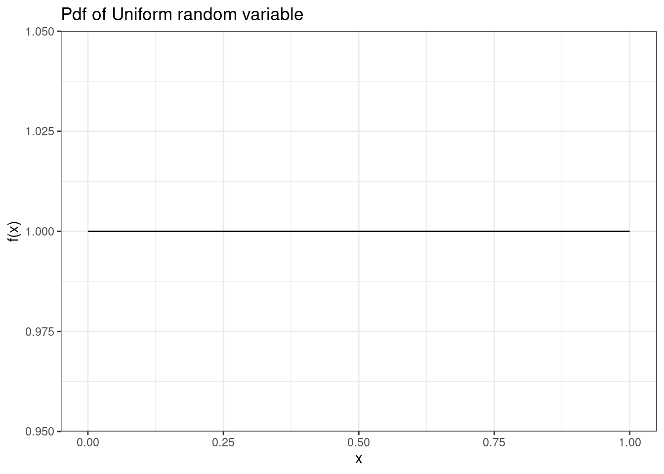
Figure 13.1: The pdf of Uniform random variable.

To check that it is a proper pdf, all values must be non-negative and the total probability must be 1. In R the function for probability density will start with the letter d and have some short descriptor for the distribution. For the uniform we use dunif().

integrate(function(x)dunif(x),0,1)

## 1 with absolute error < 1.1e-14

13.2.2 Exponential distribution

Recall from the chapter on named discrete distributions, we discussed the Poisson process. If arrivals follow a Poisson process, we know that the number of arrivals in a specified amount of time follows a Poisson distribution, and the time until the next arrival follows the exponential distribution. In the Poisson distribution, the number of arrivals is random and the interval is fixed. In the exponential distribution we change this, the interval is random and the arrivals are fixed at 1. This is a subtle point but worth the time to make sure you understand.

Let \(X\) be the number of arrivals in a time interval \(T\), where arrivals occur according to a Poisson process with an average of \(\lambda\) arrivals per unit time interval. From the previous chapter, we know that \(X\sim \textsf{Poisson}(\lambda T)\). Now let \(Y\) be the time until the next arrival. Then \(Y\) follows the exponential distribution with parameter \(\lambda\) which has units of inverse base time:

\[ Y \sim \textsf{Expon}(\lambda) \]

Note on \(\lambda\): One point of confusion involving the parameters of the Poisson and exponential distributions. The parameter of the Poisson distribution (usually denoted as \(\lambda\)) represents the average number of arrivals in whatever amount of time specified by the random variable. In the case of the exponential distribution, the parameter (also denoted as \(\lambda\)) represents the average number of arrivals per unit time. For example, suppose arrivals follow a Poisson process with an average of 10 arrivals per day. \(X\), the number of arrivals in 5 days, follows a Poisson distribution with parameter \(\lambda=50\), since that is the average number of arrivals in the amount of time specified by \(X\). Meanwhile, \(Y\), the time in days until the next arrival, follows an exponential distribution with parameter \(\lambda=10\) (the average number of arrivals per day).

The pdf of \(Y\) is given by:

\[ f_Y(y)=\lambda e^{-\lambda y}, \hspace{0.3cm} y>0 \]

The mean and variance of \(Y\) are: \(\mbox{E}(Y)=\frac{1}{\lambda}\) and \(\mbox{Var}(Y)=\frac{1}{\lambda^2}\). You should be able to derive these results but they require integration by parts and can be lengthy algebraic exercises.

Example:
Suppose at a local retail store, customers arrive to a checkout counter according to a Poisson process with an average of one arrival every three minutes. Let \(Y\) be the time (in minutes) until the next customer arrives to the counter. What is the distribution (and parameter) of \(Y\)? What are \(\mbox{E}(Y)\) and \(\mbox{Var}(Y)\)? Find \(\mbox{P}(Y>5)\), \(\mbox{P}(Y\leq 3)\), and \(\mbox{P}(1 \leq Y < 5)\)? Also, find the median and 95th percentile of \(Y\). Finally, plot the pdf of \(Y\).

Since one arrival shows up every three minutes, the average number of arrivals per unit time is 1/3 arrival per minute. Thus, \(Y\sim \textsf{Expon}(\lambda=1/3)\). This means that \(\mbox{E}(Y)=3\) and \(\mbox{Var}(Y)=9\).

To find \(\mbox{P}(Y>5)\), we could integrate the pdf of \(Y\):

\[ \mbox{P}(Y>5)=\int_5^\infty \frac{1}{3}e^{-\frac{1}{3}y}\mathop{}\!\mathrm{d}y = \lim_{a \to +\infty}\int_5^a \frac{1}{3}e^{-\frac{1}{3}y}\mathop{}\!\mathrm{d}y = \]

\[ \lim_{a \to +\infty} -e^{-\frac{1}{3}y}\bigg|_5^a=\lim_{a \to +\infty} -e^{-\frac{a}{3}}-(-e^{-\frac{5}{3}})= 0 + 0.189 = 0.189 \]

Alternatively, we could use R:

##Prob(Y>5)=1-Prob(Y<=5)
1-pexp(5,1/3)

## [1] 0.1888756

Or using integrate()

integrate(function(x)1/3*exp(-1/3*x),5,Inf)

## 0.1888756 with absolute error < 8.5e-05

For the remaining probabilities, we will use R:

##Prob(Y<=3)
pexp(3,1/3)

## [1] 0.6321206

##Prob(1<=Y<5)
pexp(5,1/3)-pexp(1,1/3)

## [1] 0.5276557

The median is \(y\) such that \(\mbox{P}(Y\leq y)=0.5\). We can find this by solving the following for \(y\): \[ \int_0^y \frac{1}{3}e^{-\frac{1}{3}y}\mathop{}\!\mathrm{d}y = 0.5 \]

Alternatively, we can use qexp in R:

##median
qexp(0.5,1/3)

## [1] 2.079442

##95th percentile
qexp(0.95,1/3)

## [1] 8.987197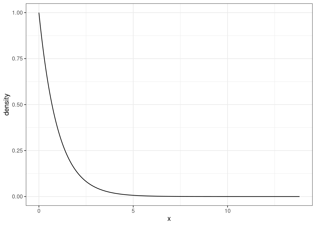

Figure 13.2: pdf of exponential random varible \(Y\)

Both from Figure 13.2 and the mean and median, we know that the exponential distribution is skewed to the right.

13.2.3 Memory-less property

The Poisson process is known for its memory-less property. Essentially, this means that the time until the next arrival is independent of the time since last arrival. Thus, the probability of an arrival within the next 5 minutes is the same regardless of whether an arrival just occurred or an arrival has not occurred for a long time.

To show this let’s consider random variable \(Y\) ( time until the next arrival in minutes) where \(Y\sim\textsf{Expon}(\lambda)\). We will show that, given it has been at least \(t\) minutes since the last arrival, the probability we wait at least \(y\) additional minutes is equal to the marginal probability that we wait \(y\) additional minutes.

First, note that the cdf of \(Y\), \(F_Y(y)=\mbox{P}(Y\leq y)=1-e^{-\lambda y}\), you should be able to derive this. So, \[ \mbox{P}(Y\geq y+t|Y\geq t) = \frac{\mbox{P}(Y\geq y+t \cap Y\geq t)}{\mbox{P}(Y\geq t)}=\frac{\mbox{P}(Y\geq y +t)}{\mbox{P}(Y\geq t)} = \frac{1-(1-e^{-(y+t)\lambda})}{1-(1-e^{-t\lambda})} \] \[ =\frac{e^{-\lambda y }e^{-\lambda t}}{e^{-\lambda t }}=e^{-\lambda y} = 1-(1-e^{-\lambda y})=\mbox{P}(Y\geq y). \blacksquare \]

Let’s simulate values for a Poisson. The Poisson is often used in modeling customer service situations such as service at Chipotle. However, some people have the mistaken idea that arrivals will be equally spaced. In fact, arrivals will come in clusters and bunches. Maybe this is the root of the common expression, “Bad news comes in threes”?

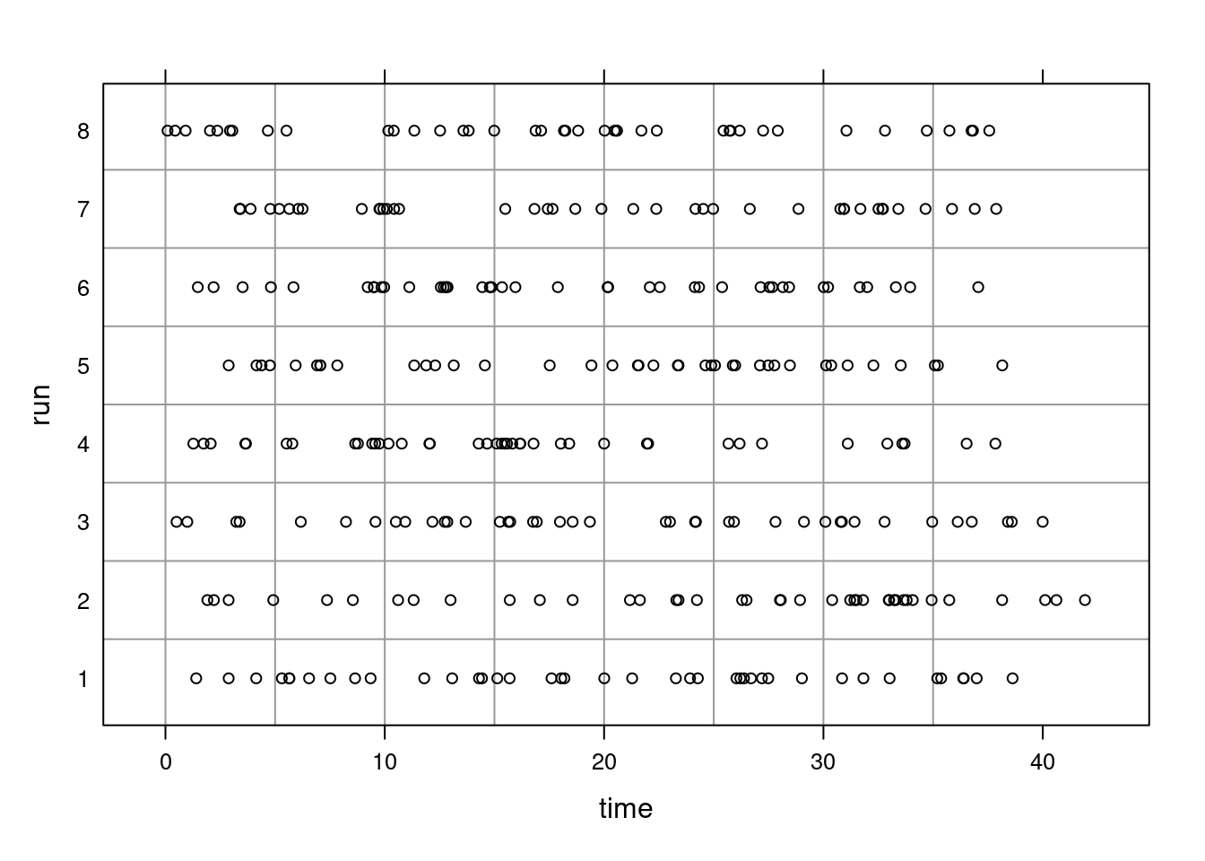
Figure 13.3: Simulations of Poisson random variable.

In Figure 13.3, the number of events in a box is \(X\sim \textsf{Poisson}(\lambda = 5)\). As you can see, some boxes have more than 5 and some less because 5 is the average number of arrivals. Also note that the spacing is not equal. The 8 different runs are just repeated simulations of the same process. We can see spacing and clusters in each run.

13.2.4 Gamma distribution

The gamma distribution is a generalization of the exponential distribution. In the exponential distribution, the parameter \(\lambda\) is sometimes referred to as the rate parameter. The gamma distribution is sometimes used to model wait times (as with the exponential distribution), but in cases without the memory-less property. The gamma distribution has two parameters, rate and shape. In some texts, scale (the inverse of rate) is used as an alternative parameter to rate.

Suppose \(X\) is a random variable with the gamma distribution with shape parameter \(\alpha\) and rate parameter \(\lambda\): \[ X \sim \textsf{Gamma}(\alpha,\lambda) \]

\(X\) has the following pdf: \[ f_X(x)=\frac{\lambda^\alpha}{\Gamma (\alpha)}x^{\alpha-1}e^{-\lambda x}, \hspace{0.3cm} x>0 \]

and 0 otherwise. The mean and variance of \(X\) are \(\mbox{E}(X)=\frac{\alpha}{\lambda}\) and \(\mbox{Var}(X)=\frac{\alpha}{\lambda^2}\). Looking at the pdf, the mean and the variance, one can easily see that if \(\alpha=1\), the resulting distribution is equivalent to \(\textsf{Expon}(\lambda)\).

13.2.4.1 Gamma function

You may have little to no background with the Gamma function (\(\Gamma (\alpha)\)). This is different from the gamma distribution. The gamma function is simply a function and is defined by:

\[ \Gamma (\alpha)=\int_0^\infty t^{\alpha-1}e^{-t}\mathop{}\!\mathrm{d}t \]

There are some important properties of the gamma function. Notably, \(\Gamma (\alpha)=(\alpha-1)\Gamma (\alpha -1)\), and if \(\alpha\) is a non-negative integer, \(\Gamma(\alpha)=(\alpha-1)!\).

Suppose \(X \sim \textsf{Gamma}(\alpha,\lambda)\). The pdf of \(X\) for various values of \(\alpha\) and \(\lambda\) is shown in Figure 13.4.

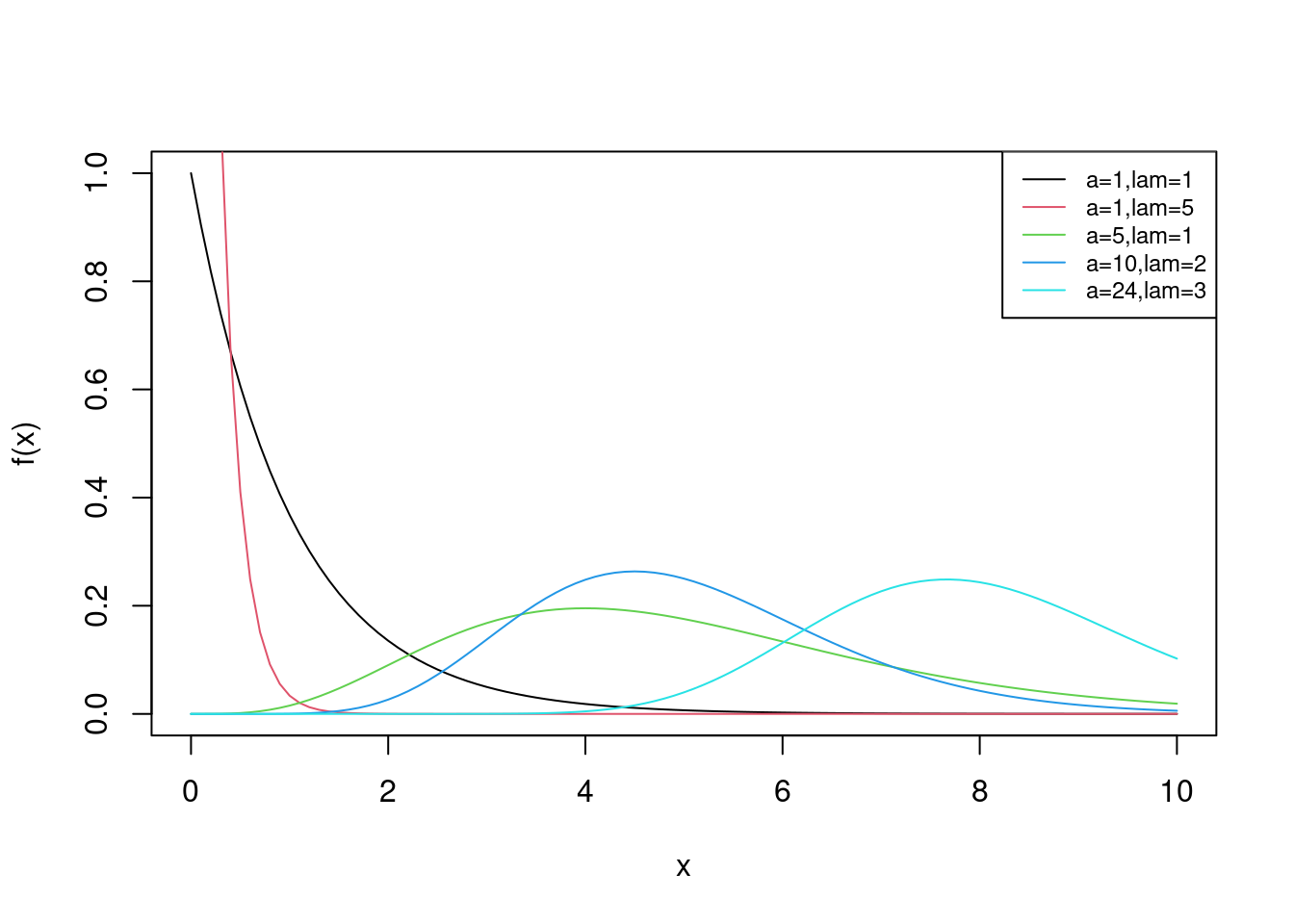
Figure 13.4: pdf of Gamma for various values of alpha and lambda

Example:
Let \(X \sim \textsf{Gamma}(\alpha=5,\lambda=1)\). Find the mean and variance of \(X\). Also, compute \(\mbox{P}(X\leq 2)\) and \(\mbox{P}(1\leq X < 8)\). Find the median and 95th percentile of \(X\).

The mean and variance of \(X\) are \(\mbox{E}(X)=5\) and \(\mbox{Var}(X)=5\). To find probabilities and quantiles, integration will be difficult, so it’s best to use the built-in R functions:

## Prob(X<=2)
pgamma(2,5,1)

## [1] 0.05265302

##Prob(1 <= X < 8)
pgamma(8,5,1)-pgamma(1,5,1)

## [1] 0.8967078

## median
qgamma(0.5,5,1)

## [1] 4.670909

## 95th percentile
qgamma(0.95,5,1)

## [1] 9.153519

13.2.5 Weibull distribution

Another common distribution used in modeling is the Weibull distribution. Like the gamma, the Weibull distribution is a generalization of the exponential distribution and is meant to model wait times. A random variable with the Weibull distribution has parameters \(\alpha\) and \(\beta\). In R, these are referred to as shape and scale respectively. Note that in some resources, these are represented by \(k\) and \(\lambda\) or even \(k\) and \(\theta\). Let \(X \sim \textsf{Weibull}(\alpha,\beta)\). The pdf of \(X\) is given by: \[ f_X(x)=\frac{\alpha}{\beta} \left(\frac{x}{\beta}\right)^{\alpha-1} e^{-\left(\frac{x}{\beta}\right)^\alpha}, \hspace{0.3cm} x\geq 0 \]

The mean and variance of a random variable with a Weibull distribution can be found by consulting R documentation. Look them up and make sure you can use them.

13.2.6 Normal distribution

The normal distribution (also referred to as Gaussian) is a common distribution found in natural processes. You have likely seen a bell curve in various contexts. The bell curve is often indicative of an underlying normal distribution. There are two parameters of the normal distribution: \(\mu\) (the mean of \(X\)) and \(\sigma\) (the standard deviation of \(X\)).

Suppose a random variable \(X\) has a normal distribution with parameters \(\mu\) and \(\sigma\). The pdf of \(X\) is given by:

\[ f_X(x)=\frac{1}{\sigma\sqrt{2\pi}}e^{-\frac{(x-\mu)^2}{2\sigma^2}}, \hspace{0.3cm} -\infty < x <\infty \]

Some plots of normal distributions for different parameters are plotted in Figure 13.5.

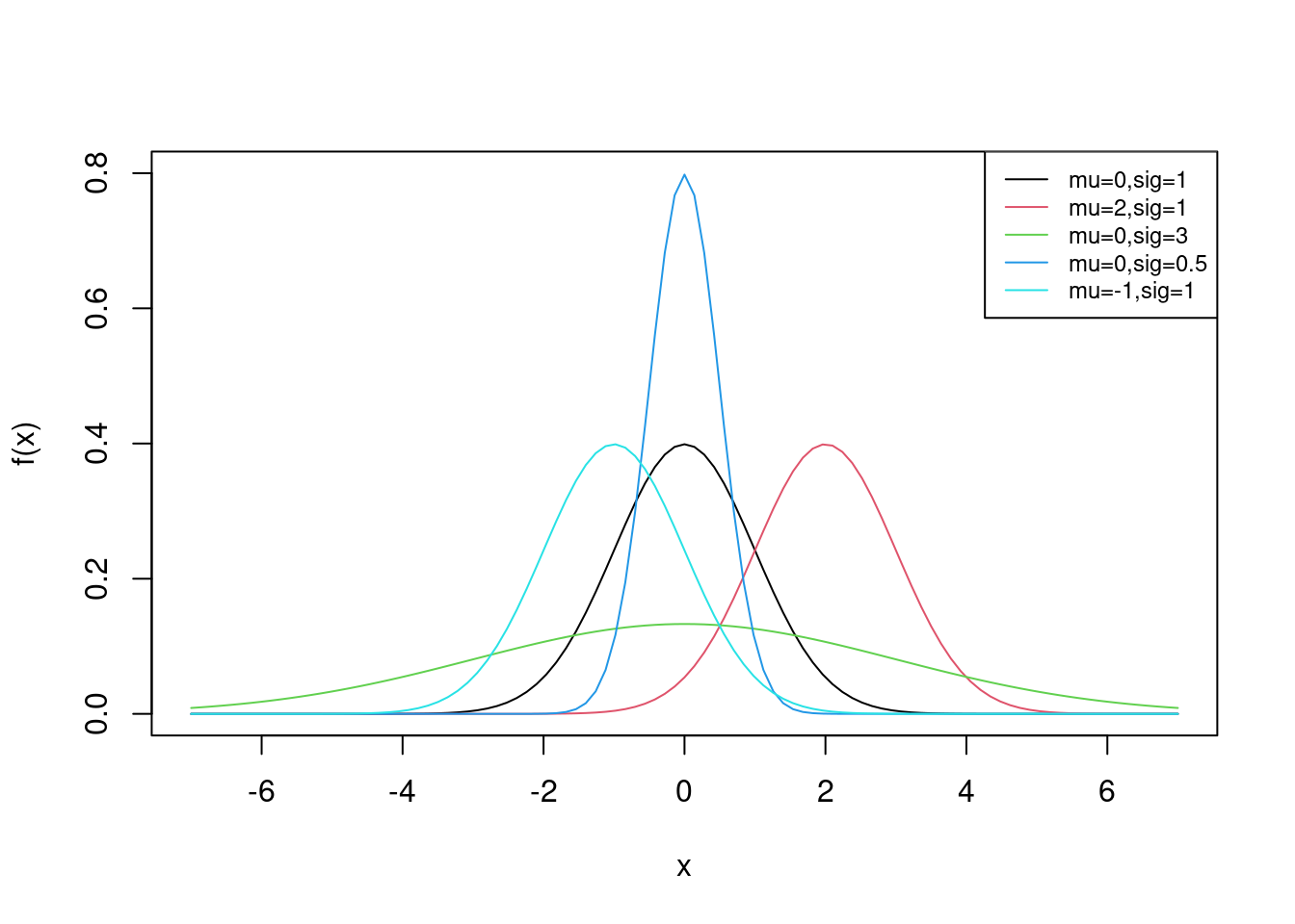
Figure 13.5: pdf of Normal for various values of mu and sigma

13.2.6.1 Standard normal

When random variable \(X\) is normally distributed with \(\mu=0\) and \(\sigma=1\), \(X\) is said to follow the standard normal distribution. Sometimes, the standard normal pdf is denoted by \(\phi(x)\).

Note that any normally distributed random variable can be transformed to have the standard normal distribution. Let \(X \sim \textsf{Norm}(\mu,\sigma)\). Then, \[ Z=\frac{X-\mu}{\sigma} \sim \textsf{Norm}(0,1) \]

Partially, one can show this is true by noting that the mean of \(Z\) is 0 and the variance (and standard deviation) of \(Z\) is 1: \[ \mbox{E}(Z)=\mbox{E}\left(\frac{X-\mu}{\sigma}\right)=\frac{1}{\sigma}\left(\mbox{E}(X)-\mu\right)=\frac{1}\sigma(\mu-\mu)=0 \] \[ \mbox{Var}(Z)=\mbox{Var}\left(\frac{X-\mu}{\sigma}\right)=\frac{1}{\sigma^2}\left(\mbox{Var}(X)-0\right)=\frac{1}{\sigma^2} \sigma^2=1 \]

Note that this does not prove that \(Z\) follows the standard normal distribution; we have merely shown that \(Z\) has a mean of 0 and a variance of 1. We will discuss transformation of random variables in a later chapter.

Example:
Let \(X \sim \textsf{Norm}(\mu=200,\sigma=15)\). Compute \(\mbox{P}(X\leq 160)\), \(\mbox{P}(180\leq X < 230)\), and \(\mbox{P}(X>\mu+\sigma)\). Find the median and 95th percentile of \(X\).

As with the gamma distribution, to find probabilities and quantiles, integration will be difficult, so it’s best to use the built-in R functions:

## Prob(X<=160)
pnorm(160,200,15)

## [1] 0.003830381

##Prob(180 <= X < 230)
pnorm(230,200,15)-pnorm(180,200,15)

## [1] 0.8860386

##Prob(X>mu+sig)
1-pnorm(215,200,15)

## [1] 0.1586553

## median
qnorm(0.5,200,15)

## [1] 200

## 95th percentile
qnorm(0.95,200,15)

## [1] 224.6728

13.2.7 Beta distribution

The last common continuous distribution we will study is the beta distribution. This has a unique application in that the domain of a random variable with the beta distribution is \([0,1]\). Thus it is typically used to model proportions. The beta distribution has two parameters, \(\alpha\) and \(\beta\). (In R, these are denoted not so cleverly as shape1 and shape2.)

Let \(X \sim \textsf{Beta}(\alpha,\beta)\). The pdf of \(X\) is given by: \[ f_X(x)=\frac{\Gamma(\alpha + \beta)}{\Gamma(\alpha)\Gamma(\beta)}x^{\alpha-1}(1-x)^{\beta-1}, \hspace{0.3cm} 0\leq x \leq 1 \]

Yes, our old friend the Gamma function. In some resources, \(\frac{\Gamma(\alpha + \beta)}{\Gamma(\alpha)\Gamma(\beta)}\) is written as \(\frac{1}{B(\alpha,\beta)}\), where \(B\) is known as the beta function.

Note that \(\mbox{E}(X)=\frac{\alpha}{\alpha+\beta}\) and \(\mbox{Var}(X)=\frac{\alpha \beta}{(\alpha+\beta)^2(\alpha+\beta+1)}\).

For various values \(\alpha\) and \(\beta\), the pdf of a beta distributed random variable is shown in Figure 13.6.

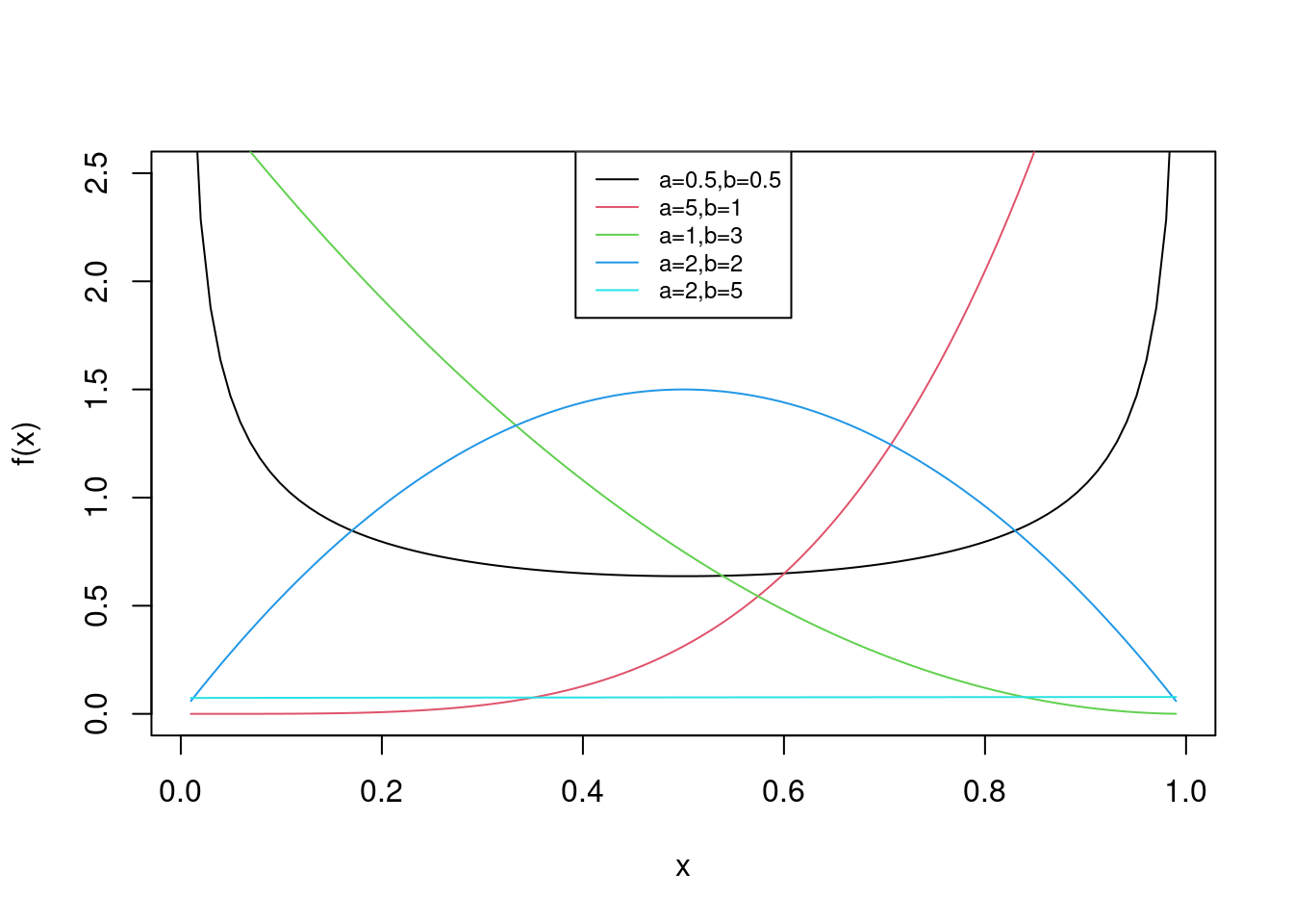
Figure 13.6: pdf of Beta for various values of alpha and beta

Exercise
What is the distribution if \(\alpha=\beta=1\)?

It is the uniform. It is easy to verify that \(\Gamma(1)=1\) so that \(B(1,1)=1\).

13.3 Homework Problems

For problems 1-3 below, 1) define a random variable that will help you answer the question, 2) state the distribution and parameters of that random variable; 3) determine the expected value and variance of that random variable, and 4) use that random variable to answer the question.

1. On a given Saturday, suppose vehicles arrive at the USAFA North Gate according to a Poisson process at a rate of 40 arrivals per hour.

1. Find the probability no vehicles arrive in 10 minutes.
   
2. Find the probability that at least 5 minutes will pass before the next arrival.
   
3. Find the probability that the next vehicle will arrive between 2 and 10 minutes from now.
   
4. Find the probability that at least 7 minutes will pass before the next arrival, given that 2 minutes have already passed. Compare this answer to part (b). This is an example of the memory-less property of the exponential distribution.
   
5. Fill in the blank. There is a probability of 90% that the next vehicle will arrive within __ minutes. This value is known as the 90% percentile of the random variable.
   
6. Use the function stripplot() to visualize the arrival of 30 vehicles using a random sample from the appropriate exponential distribution.

2. Suppose time until computer errors on the F-35 follows a Gamma distribution with mean 20 hours and variance 10.

1. Find the probability that 20 hours pass without a computer error.
   
2. Find the probability that 45 hours pass without a computer error, given that 25 hours have already passed. Does the memory-less property apply to the Gamma distribution?
   
3. Find \(a\) and \(b\) where there is a 95% probability time until next computer error will be between \(a\) and \(b\). (note: technically, there are many answers to this question, but find \(a\) and \(b\) such that each tail has equal probability.)

3. Suppose PFT scores in the cadet wing follow a normal distribution with mean 330 and standard deviation 50.

1. Find the probability a randomly selected cadet has a PFT score higher than 450.
   
2. Find the probability a randomly selected cadet has a PFT score within 2 standard deviations of the mean.
   
3. Find \(a\) and \(b\) such that 90% of PFT scores will be between \(a\) and \(b\).
   
4. Find the probability a randomly selected cadet has a PFT score higher than 450 given he/she is among the top 10% of cadets.

4. Let \(X \sim \textsf{Beta}(\alpha=1,\beta=1)\). Show that \(X\sim \textsf{Unif}(0,1)\). Hint: write out the beta distribution pdf where \(\alpha=1\) and \(\beta=1\).

5. When using R to calculate probabilities related to the gamma distribution, we often use pgamma. Recall that pgamma is equivalent to the cdf of the gamma distribution. If \(X\sim\textsf{Gamma}(\alpha,\lambda)\), then \[ \mbox{P}(X\leq x)=\textsf{pgamma(x,alpha,lambda)} \] The dgamma function exists in R too. In plain language, explain what dgamma returns. I’m not looking for the definition found in R documentation. I’m looking for a simple description of what that function returns. Is the output of dgamma useful? If so, how?

6. Advanced. You may have heard of the 68-95-99.7 rule. This is a helpful rule of thumb that says if a population has a normal distribution, then 68% of the data will be within one standard deviation of the mean, 95% of the data will be within two standard deviations and 99.7% of the data will be within three standard deviations. Create a function in R that has two inputs (a mean and a standard deviation). It should return a vector with three elements: the probability that a randomly selected observation from the normal distribution with the inputted mean and standard deviation lies within one, two and three standard deviations. Test this function with several values of the mu and sd. You should get the same answer each time.

7. Derive the mean of a general uniform distribution, \(U(a,b)\).

Solutions Manual