10 Random Variables

10.1 Objectives

Define and use properly in context all new terminology, to include: random variable, discrete random variable, continuous random variable, mixed random variable, distribution function, probability mass function, cumulative distribution function, moment, expectation, mean, variance.
Given a discrete random variable, obtain the pmf and cdf, and use them to obtain probabilities of events.
Simulate random variables for a discrete distribution.
Find the moments of a discrete random variable.
Find the expected value of a linear transformation of a random variable.

10.2 Random variables

We have already discussed random experiments. We have also discussed \(S\), the sample space for an experiment. A random variable essentially maps the events in the sample space to the real number line. For a formal definition: A random variable \(X\) is a function \(X: S\rightarrow \mathbb{R}\) that assigns exactly one number to each outcome in an experiment.

Example:
Suppose you flip a coin three times. The sample space, \(S\), of this experiment is \[ S=\{\mbox{HHH}, \mbox{HHT}, \mbox{HTH}, \mbox{HTT}, \mbox{THH}, \mbox{THT}, \mbox{TTH}, \mbox{TTT}\} \]

Let the random variable \(X\) be the number of heads in three coin flips. Whenever introduced to a new random variable, you should take a moment to think about what possible values can \(X\) take? When tossing a coin 3 times, we can get no heads, one head, two heads or three heads. The random variable \(X\) assigns each outcome in our experiment to one of these values. Visually: \[ S=\{\underbrace{\mbox{HHH}}_{X=3}, \underbrace{\mbox{HHT}}_{X=2}, \underbrace{\mbox{HTH}}_{X=2}, \underbrace{\mbox{HTT}}_{X=1}, \underbrace{\mbox{THH}}_{X=2}, \underbrace{\mbox{THT}}_{X=1}, \underbrace{\mbox{TTH}}_{X=1}, \underbrace{\mbox{TTT}}_{X=0}\} \]

The sample space of \(X\), sometimes referred to as the support, is the list of numerical values that \(X\) can take. \[ S_X=\{0,1,2,3\} \]

Because the sample space of \(X\) is a countable list of numbers, we consider \(X\) to be a discrete random variable (more on that later).

10.2.1 How does this help?

Sticking with our example, we can now frame a problem of interest in the context of our random variable \(X\). For example, suppose we wanted to know the probability of at least two heads. Without our random variable, we have to write this as: \[ \mbox{P}(\mbox{at least two heads})= \mbox{P}(\{\mbox{HHH},\mbox{HHT},\mbox{HTH},\mbox{THH}\}) \]

In the context of our random variable, this simply becomes \(\mbox{P}(X\geq 2)\). It may not seem important in a case like this, but imagine if we were flipping a coin 50 times and wanted to know the probability of obtaining at least 30 heads. It would be unfeasible to write out all possible ways to obtain at least 30 heads. It is much easier to write \(\mbox{P}(X\geq 30)\) and explore the distribution of \(X\).

Essentially, a random variable often helps us reduce a complex random experiment to a simple variable that is easy to characterize.

10.2.2 Discrete vs Continuous

A discrete random variable has a sample space that consists of a countable set of values. \(X\) in our example above is a discrete random variable. Note that “countable” does not necessarily mean “finite”. For example, a random variable with a Poisson distribution (a topic for a later chapter) has a sample space of \(\{0,1,2,...\}\). This sample space is unbounded, but it is considered countably infinite, and thus the random variable would be considered discrete.

A continuous random variable has a sample space that is a continuous interval. For example, let \(Y\) be the random variable corresponding to the height of a randomly selected individual. \(Y\) is a continuous random variable because a person could measure 68.1 inches, 68.2 inches, or perhaps any value in between. Note that when we measure height, our precision is limited by our measuring device, so we are technically “discretizing” height. However, even in these cases, we typically consider height to be a continuous random variable.

A mixed random variable is exactly what it sounds like. It has a sample space that is both discrete and continuous. How could such a thing occur? Consider an experiment where a person rolls a standard six-sided die. If it lands on anything other than one, the result of the die roll is recorded. If it lands on one, the person spins a wheel, and the angle in degrees of the resulting spin, divided by 360, is recorded. If our random variable \(Z\) is the number that is recorded in this experiment, the sample space of \(Z\) is \([0,1] \cup \{2,3,4,5,6\}\). We will not be spending much time on mixed random variables. However they do occur in practice, consider the job of analyzing bomb error data. If the bomb hits within a certain radius, the error is 0. Otherwise it is measured in a radial direction. This data is mixed.

10.2.3 Discrete distribution functions

Once we have defined a random variable, we need a way to describe its behavior and we will use probabilities for this purpose.

Distribution functions describe the behavior of random variables. We can use these functions to determine the probability that a random variable takes a value or a range of values. For discrete random variables, there are two distribution functions of interest: the probability mass function (pmf) and the cumulative distribution function (cdf).

10.2.4 Probability mass function

Let \(X\) be a discrete random variable. The probability mass function (pmf) of \(X\), given by \(f_X(x)\), is a function that assigns probability to each possible outcome of \(X\). \[ f_X(x)=\mbox{P}(X=x) \]

Note that the pmf is a function. Functions have input and output. The input of a pmf is any real number. The output of a pmf is the probability that the random variable takes the inputted value. The pmf must follow the axioms of probability described in the Probability Rules chapter. Primarily,

For all \(x \in \mathbb{R}\), \(0 \leq f_X(x) \leq 1\).
\(\sum_x f_X(x) = 1\), where the \(x\) in the index of the sum simply denotes that we are summing across the entire domain or support of \(X\).

Example:
Recall our example again. You flip a coin three times and let \(X\) be the number of heads in those three coin flips. We know that \(X\) can only take values 0, 1, 2 or 3. But at what probability does it take these three values? In that example, we had listed out the possible outcomes of the experiment and denoted what value of \(X\) corresponds to each outcome. \[ S=\{\underbrace{\mbox{HHH}}_{X=3}, \underbrace{\mbox{HHT}}_{X=2}, \underbrace{\mbox{HTH}}_{X=2}, \underbrace{\mbox{HTT}}_{X=1}, \underbrace{\mbox{THH}}_{X=2}, \underbrace{\mbox{THT}}_{X=1}, \underbrace{\mbox{TTH}}_{X=1}, \underbrace{\mbox{TTT}}_{X=0}\} \]

Each of these eight outcomes is equally likely (each with a probability of \(\frac{1}{8}\)). Thus, building the pmf of \(X\) becomes a matter of counting the number of outcomes associated with each possible value of \(X\): \[ f_X(x)=\left\{ \renewcommand{\arraystretch}{1.4} \begin{array}{ll} \frac{1}{8}, & x=0 \\ \frac{3}{8}, & x=1 \\ \frac{3}{8}, & x=2 \\ \frac{1}{8}, & x=3 \\ 0, & \mbox{otherwise} \end{array} \right . \]

Note that this function specifies the probability that \(X\) takes any of the four values in the sample space (0, 1, 2, and 3). Also, it specifies that the probability that \(X\) takes any other value is 0.

Graphically, the pmf is not terribly interesting. The pmf is 0 at all values of \(X\) except for 0, 1, 2 and 3, Figure 10.1.

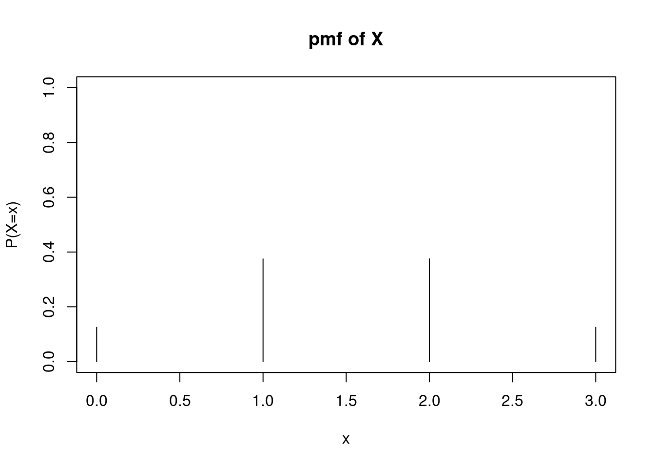
Figure 10.1: Probability Mass Function of \(X\) from Coin Flip Example

Example:
We can use a pmf to answer questions about an experiment. For example, consider the same context. What is the probability that we flip at least one heads? We can write this in the context of \(X\): \[ \mbox{P}(\mbox{at least one heads})=\mbox{P}(X\geq 1)=\mbox{P}(X=1)+\mbox{P}(X=2)+\mbox{P}(X=3)=\frac{3}{8} + \frac{3}{8}+\frac{1}{8}=\frac{7}{8} \]

Alternatively, we can recognize that \(\mbox{P}(X\geq 1)=1-\mbox{P}(X=0)=1-\frac{1}{8}=\frac{7}{8}\).

10.2.5 Cumulative distribution function

Let \(X\) be a discrete random variable. The cumulative distribution function (cdf) of \(X\), given by \(F_X(x)\), is a function that assigns to each value of \(X\) the probability that \(X\) takes that value or lower: \[ F_X(x)=\mbox{P}(X\leq x) \]

Again, note that the cdf is a function with an input and output. The input of a cdf is any real number. The output of a cdf is the probability that the random variable takes the inputted value or less.

If we know the pmf, we can obtain the cdf: \[ F_X(x)=\mbox{P}(X\leq x)=\sum_{y\leq x} f_X(y) \]

Like the pmf, the cdf must be between 0 and 1. Also, since the pmf is always non-negative, the cdf must be non-decreasing.

Example:
Obtain and plot the cdf of \(X\) of the previous example. \[ F_X(x)=\mbox{P}(X\leq x)=\left\{\renewcommand{\arraystretch}{1.4} \begin{array}{ll} 0, & x <0 \\ \frac{1}{8}, & 0\leq x < 1 \\ \frac{4}{8}, & 1\leq x < 2 \\ \frac{7}{8}, & 2\leq x < 3 \\ 1, & x\geq 3 \end{array}\right . \]

Visually, the cdf of a discrete random variable has a stairstep appearance. In this example, the cdf takes a value 0 up until \(X=0\), at which point the cdf increases to 1/8. It stays at this value until \(X=1\), and so on. At and beyond \(X=3\), the cdf is equal to 1, Figure 10.2.

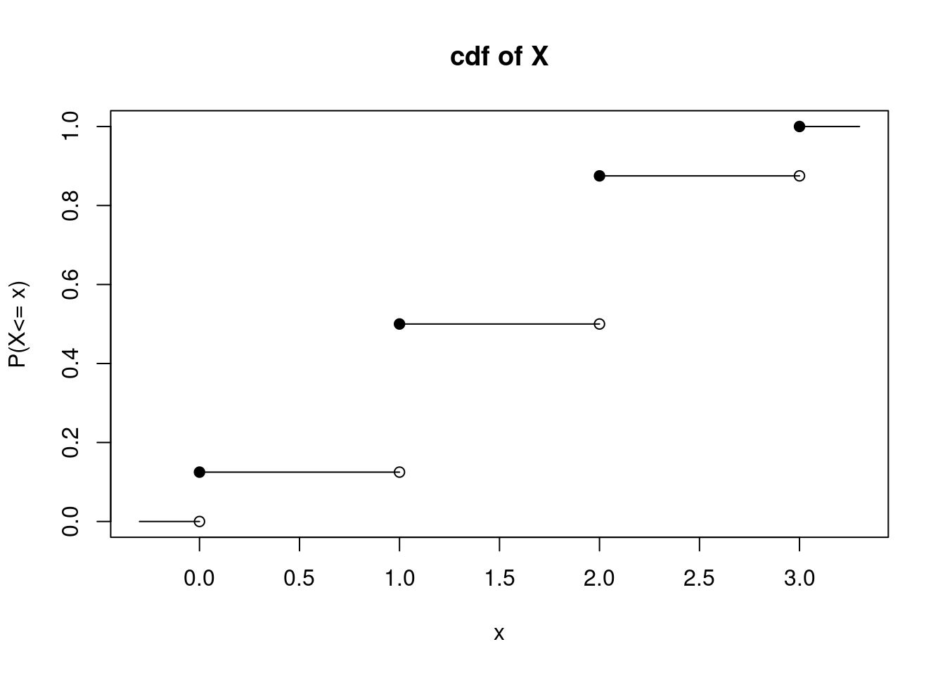
Figure 10.2: Cumulative Distribution Function of \(X\) from Coin Flip Example

10.2.6 Simulating random variables

We can simulate values from a random variable using the cdf, we will use a similar idea for continuous random variables. Since the range of the cdf is in the interval \([0,1]\) we will generate a random number in that same interval and then use the inverse function to find the value of the random variable. The pseudo code is:
1) Generate a random number, \(U\).
2) Find the index \(k\) such that \(\sum_{j=1}^{k-1}f_X(x_{j}) \leq U < \sum_{j=1}^{k}f_X(x_{j})\) or \(F_x(k-1) \leq U < F_{x}(k)\).

Example:
Simulate a random variable for the number of heads in flipping a coin three times.

First we will create the pmf.

pmf <- c(1/8,3/8,3/8,1/8)
values <- c(0,1,2,3)
pmf

## [1] 0.125 0.375 0.375 0.125

We get the cdf from the cumulative sum.

cdf <- cumsum(pmf)
cdf

## [1] 0.125 0.500 0.875 1.000

Next, we will generate a random number between 0 and 1.

set.seed(1153)
ran_num <- runif(1)
ran_num

## [1] 0.7381891

Finally, we will find the value of the random variable. We will do each step separately first so you can understand the code.

ran_num < cdf

## [1] FALSE FALSE  TRUE  TRUE

which(ran_num < cdf)

## [1] 3 4

which(ran_num < cdf)[1]

## [1] 3

values[which(ran_num < cdf)[1]]

## [1] 2

Let’s make this a function.

simple_rv <- function(values,cdf){
ran_num <- runif(1)
return(values[which(ran_num < cdf)[1]])
}

Now let’s generate 10000 values from this random variable.

results <- do(10000)*simple_rv(values,cdf)
inspect(results)

## 
## quantitative variables:  
##        name   class min Q1 median Q3 max   mean       sd     n missing
## 1 simple_rv numeric   0  1      2  2   3 1.5048 0.860727 10000       0

tally(~simple_rv,data=results,format="proportion")

## simple_rv
##      0      1      2      3 
## 0.1207 0.3785 0.3761 0.1247

Not a bad approximation.

10.3 Moments

Distribution functions are excellent characterizations of random variables. The pmf and cdf will tell you exactly how often the random variables takes particular values. However, distribution functions are often a lot of information. Sometimes, we may want to describe a random variable \(X\) with a single value or small set of values. For example, we may want to know the average or some measure of center of \(X\). We also may want to know a measure of spread of \(X\). Moments are values that summarize random variables with single numbers. Since we are dealing with the population, these moments are population values and not summary statistics as we used in the first block of material.

10.3.1 Expectation

At this point, we should define the term expectation. Let \(g(X)\) be some function of a discrete random variable \(X\). The expected value of \(g(X)\) is given by: \[ \mbox{E}(g(X))=\sum_x g(x) \cdot f_X(x) \]

10.3.2 Mean

The most common moments used to describe random variables are mean and variance. The mean (often referred to as the expected value of \(X\)), is simply the average value of a random variable. It is denoted as \(\mu_X\) or \(\mbox{E}(X)\). In the discrete case, the mean is found by: \[ \mu_X=\mbox{E}(X)=\sum_x x \cdot f_X(x) \]

The mean is also known as the first moment of \(X\) around the origin. It is a weighted sum with the weight being the probability. If each outcome were equally likely, the expected value would just be the average of the values of the random variable since each weight is the reciprocal of the number of values.

Example:
Find the expected value (or mean) of \(X\): the number of heads in three flips of a fair coin. \[ \mbox{E}(X)=\sum_x x\cdot f_X(x) = 0*\frac{1}{8} + 1*\frac{3}{8} + 2*\frac{3}{8} + 3*\frac{1}{8}=1.5 \]

We are using \(\mu\) because it is a population parameter.

From our simulation above, we can find the mean as an estimate of the expected value. This is really a statistic since our simulation is data from the population and thus will have variance from sample to sample.

mean(~simple_rv,data=results)

## [1] 1.5048

10.3.3 Variance

Variance is a measure of spread of a random variable. The variance of \(X\) is denoted as \(\sigma^2_X\) or \(\mbox{Var}(X)\). It is equivalent to the average squared deviation from the mean: \[ \sigma^2_X=\mbox{Var}(X)=\mbox{E}[(X-\mu_X)^2] \]

In the discrete case, this can be evaluated by: \[ \mbox{E}[(X-\mu_X)^2]=\sum_x (x-\mu_X)^2f_X(x) \]

Variance is also known as the second moment of \(X\) around the mean.

The square root of \(\mbox{Var}(X)\) is denoted as \(\sigma_X\), the standard deviation of \(X\). The standard deviation is often reported because it is measured in the same units as \(X\), while the variance is measured in squared units and is thus harder to interpret.

Example:
Find the variance of \(X\): the number of heads in three flips of a fair coin.

\[ \mbox{Var}(X)=\sum_x (x-\mu_X)^2 \cdot f_X(x) \]

\[ = (0-1.5)^2 \times \frac{1}{8} + (1-1.5)^2 \times \frac{3}{8}+(2-1.5)^2 \times \frac{3}{8} + (3-1.5)^2\times \frac{1}{8} \] In R this is:

(0-1.5)^2*1/8 + (1-1.5)^2*3/8 + (2-1.5)^2*3/8 + (3-1.5)^2*1/8

## [1] 0.75

The variance of \(X\) is 0.75.

We can find the variance of the simulation but R uses the sample variance and this is the population variance. So we need to multiply by \(\frac{n-1}{n}\)

var(~simple_rv,data=results)*(10000-1)/10000

## [1] 0.740777

10.3.4 Mean and variance of Linear Transformations

Lemma: Let \(X\) be a discrete random variable, and let \(a\) and \(b\) be constants. Then: \[ \mbox{E}(aX+b)=a\mbox{E}(X)+b \] and \[ \mbox{Var}(aX+b)=a^2\mbox{Var}(X) \]

The proof of this is left as a homework problem.

10.4 Homework Problems

Suppose we are flipping a fair coin, and the result of a single coin flip is either heads or tails. Let \(X\) be a random variable representing the number of flips until the first heads.

Is \(X\) discrete or continuous? What is the domain, support, of \(X\)?
What values do you expect \(X\) to take? What do you think is the average of \(X\)? Don’t actually do any formal math, just think about if you were flipping a regular coin, how long it would take you to get the first heads.
Advanced: In R, generate 10,000 observations from \(X\). What is the empirical, from the simulation, pmf? What is the average value of \(X\) based on this simulation? Create a bar chart of the proportions. Note: Unlike the example in the Notes, we don’t have the pmf, so you will have to simulate the experiment and using R to find the number of flips until the first heads.

Note: There are many ways to do this. Below is a description of one approach. It assumes we are extremely unlikely to go past 1000 flips.

First, let’s sample with replacement from the vector c(“H”,“T”), 1000 times with replacement, use sample().
As we did in the reading, use which() and a logical argument to find the first occurrence of a heads.

Find the theoretical distribution, use math to come up with a closed for solution for the pmf.

Repeat Problem 1,except part d, but with a different random variable, \(Y\): the number of coin flips until the fifth heads.

Suppose you are a data analyst for a large international airport. Your boss, the head of the airport, is dismayed that this airport has received negative attention in the press for inefficiencies and sluggishness. In a staff meeting, your boss gives you a week to build a report addressing the “timeliness” at the airport. Your boss is in a big hurry and gives you no further information or guidance on this task.

Prior to building the report, you will need to conduct some analysis. To aid you in this, create a list of at least three random variables that will help you address timeliness at the airport. For each of your random variables,

Determine whether it is discrete or continuous.
Report its domain.
What is the experimental unit?
Explain how this random variable will be useful in addressing timeliness at the airport.

We will provide one example:

Let \(D\) be the difference between a flight’s actual departure and its scheduled departure. This is a continuous random variable, since time can be measured in fractions of minutes. A flight can be early or late, so domain is any real number. The experimental unit is each individual (non-canceled) flight. This is a useful random variable because the average value of \(D\) will describe whether flights take off on time. We could also find out how often \(D\) exceeds 0 (implying late departure) or how often \(D\) exceeds 30 minutes, which could indicate a “very late” departure.

Consider the experiment of rolling two fair six-sided dice. Let the random variable \(Y\) be the absolute difference between the two numbers that appear upon rolling the dice.

What is the domain/support of \(Y\)?
What values do you expect \(Y\) to take? What do you think is the average of \(Y\)? Don’t actually do any formal math, just think about the experiment.
Find the probability mass function and cumulative distribution function of \(Y\).
Find the expected value and variance of \(Y\).
Advanced: In R, obtain 10,000 realizations of \(Y\). In other words, simulate the roll of two fair dice, record the absolute difference and repeat this 10,000 times. Construct a frequency table of your results (what percentage of time did you get a difference of 0? difference of 1? etc.) Find the mean and variance of your simulated sample of \(Y\). Were they close to your answers in part d?

Prove the Lemma from the Notes: Let \(X\) be a discrete random variable, and let \(a\) and \(b\) be constants. Show \(\mbox{E}(aX + b)=a\mbox{E}(X)+b\).

We saw that \(\mbox{Var}(X)=\mbox{E}[(X-\mu_X)^2]\). Show that \(\mbox{Var}(X)\) is also equal to \(\mbox{E}(X^2)-[\mbox{E}(X)]^2\).

Solutions Manual

9 Conditional Probability

11 Continuous Random Variables