29 Linear Regression Diagnostics
29.1 Objectives
Obtain and interpret \(R\)-squared and the \(F\)-statistic.
Use
Rto evaluate the assumptions of a linear model.Identify and explain outliers and leverage points.
29.2 Homework
29.2.1 Problem 1
Identify relationships
For each of the six plots, identify the strength of the relationship (e.g. weak, moderate, or strong) in the data and whether fitting a linear model would be reasonable. When we ask about the strength of the relationship, we mean:
- is there a relationship between \(x\) and \(y\) and
- does that relationship explain most of the variance?
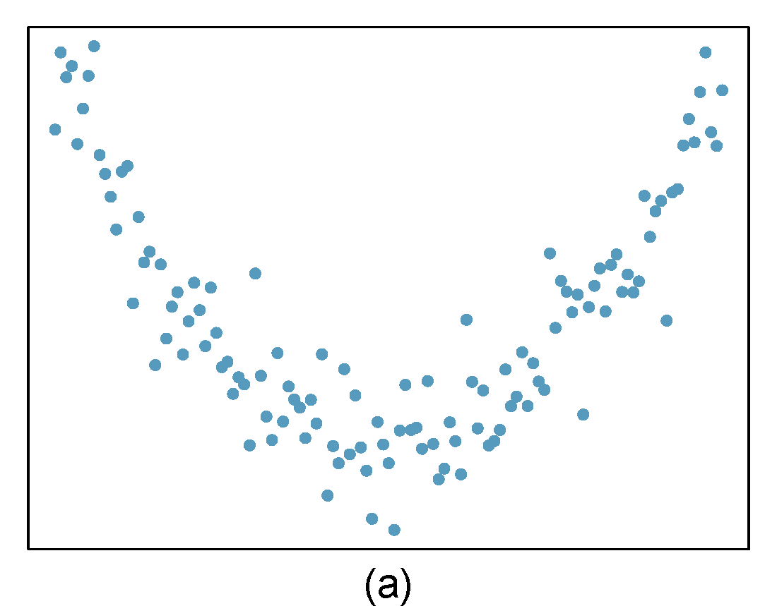
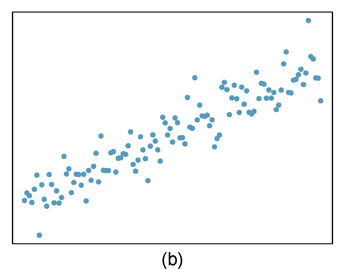
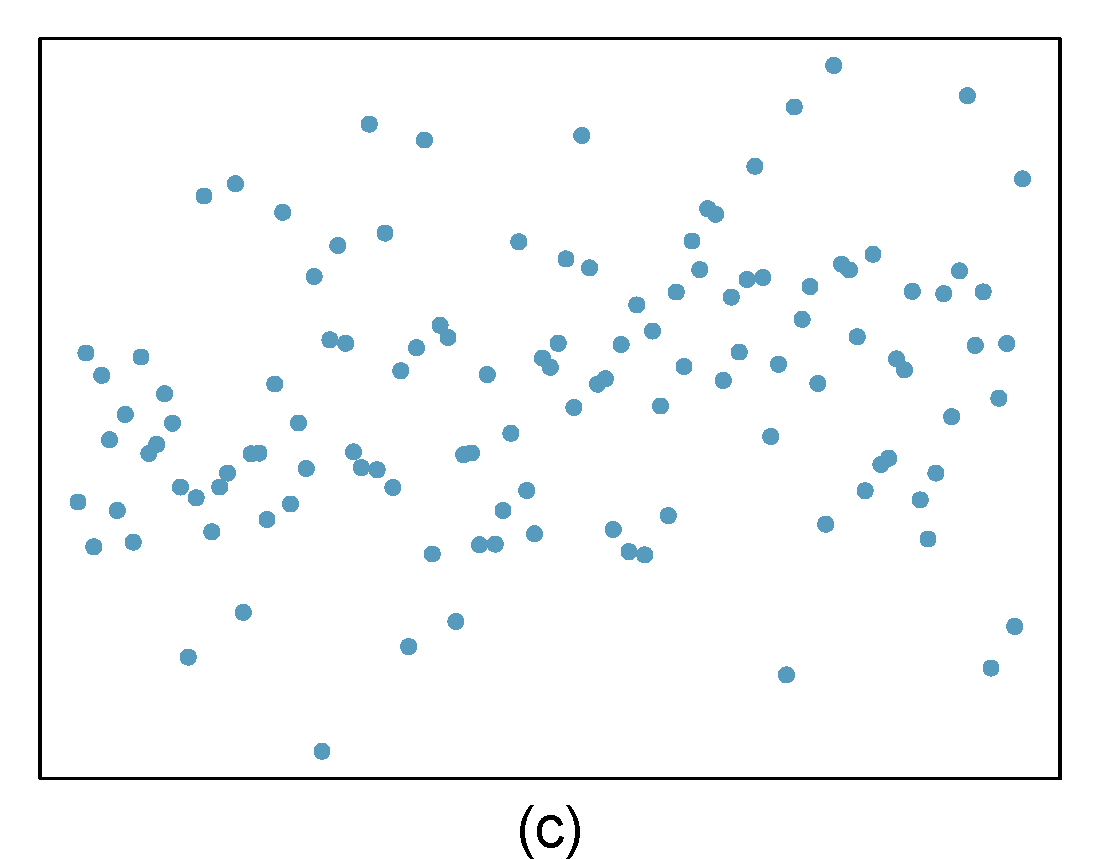
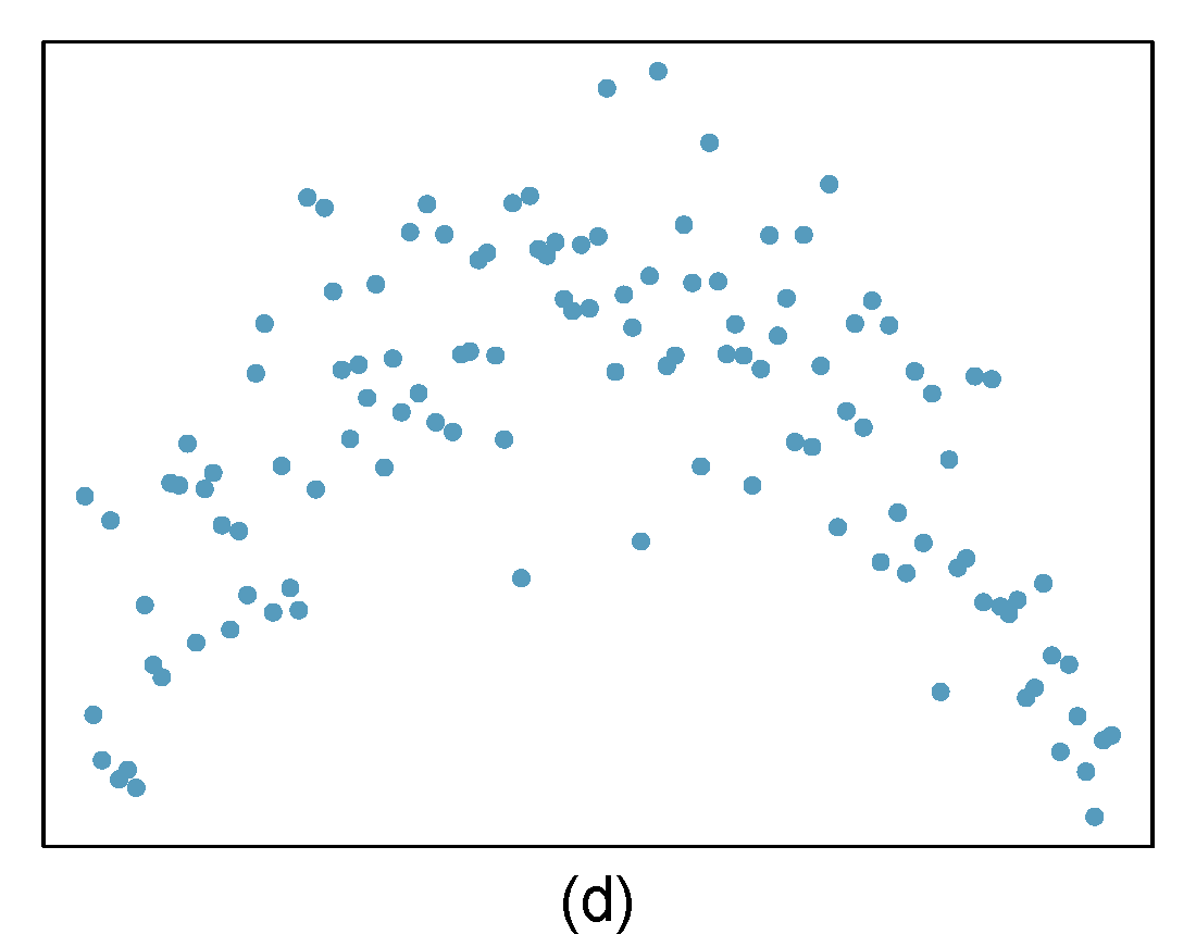
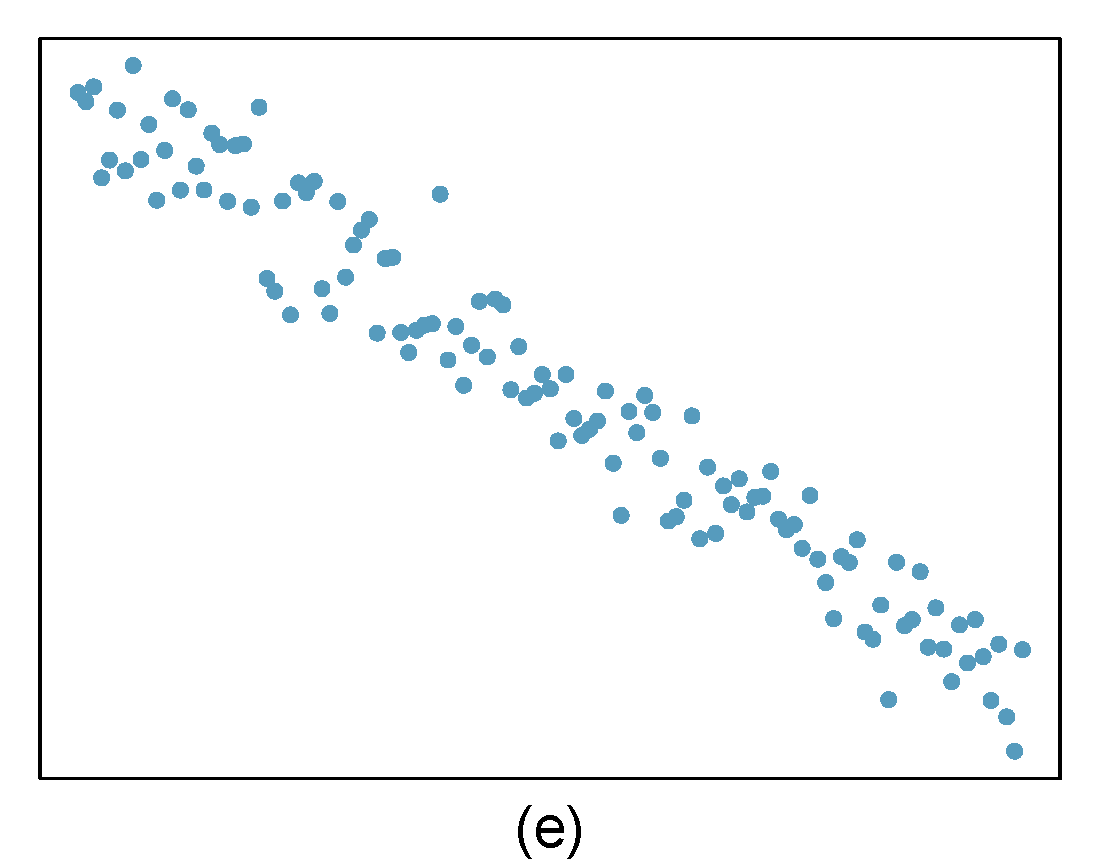
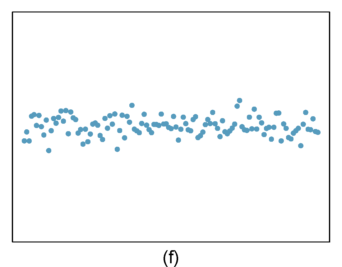
Figure 29.1: Homework problem 1.
- Strong relationship, but a straight line would not fit the data.
- Strong relationship, and a linear fit would be reasonable.
- Weak relationship, and trying a linear fit would be reasonable.
- Moderate relationship, but a straight line would not fit the data.
- Strong relationship, and a linear fit would be reasonable.
- Weak relationship because a change in \(x\) does not cause a change in \(y\) even though the points would cluster around a horizontal line. Trying a linear fit would be reasonable.
29.2.2 Problem 2
Beer and blood alcohol content
We will use the blood alcohol content data again. As a reminder this is the description of the data: Many people believe that gender, weight, drinking habits, and many other factors are much more important in predicting blood alcohol content (BAC) than simply considering the number of drinks a person consumed. Here we examine data from sixteen student volunteers at Ohio State University who each drank a randomly assigned number of cans of beer. These students were evenly divided between men and women, and they differed in weight and drinking habits. Thirty minutes later, a police officer measured their blood alcohol content (BAC) in grams of alcohol per deciliter of blood.
The data is in the bac.csv file under the data folder.
- Obtain and interpret \(R\)-squared for this model.
bac<-read_csv("data/bac.csv")
bac %>%
  gf_point(bac~beers) %>%
  gf_labs(x="Number of cans of beer",y="BAC") %>%
  gf_theme(theme_classic()) %>%
  gf_refine(scale_x_continuous(breaks = c(1,2,3,4,5,6,7,8,9)))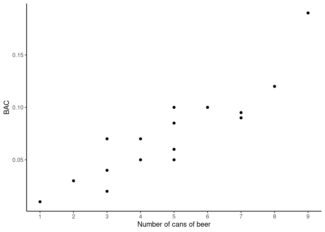
bac_mod <- lm(bac~beers,data=bac)
summary(bac_mod)##
## Call:
## lm(formula = bac ~ beers, data = bac)
##
## Residuals:
## Min 1Q Median 3Q Max
## -0.027118 -0.017350 0.001773 0.008623 0.041027
##
## Coefficients:
## Estimate Std. Error t value Pr(>|t|)
## (Intercept) -0.012701 0.012638 -1.005 0.332
## beers 0.017964 0.002402 7.480 2.97e-06 ***
## ---
## Signif. codes: 0 '***' 0.001 '**' 0.01 '*' 0.05 '.' 0.1 ' ' 1
##
## Residual standard error: 0.02044 on 14 degrees of freedom
## Multiple R-squared: 0.7998, Adjusted R-squared: 0.7855
## F-statistic: 55.94 on 1 and 14 DF, p-value: 2.969e-06The \(R\)-squared is 0.7998, this means that almost 80% of the variance in blood alcohol content is explained by the number of beers consumed. This is not surprising. The remaining variance may be due to measurement errors, differences in the students, and environmental impacts.
- Evaluate the assumptions of this model. Do we have anything to be concerned about?
plot(bac_mod,1)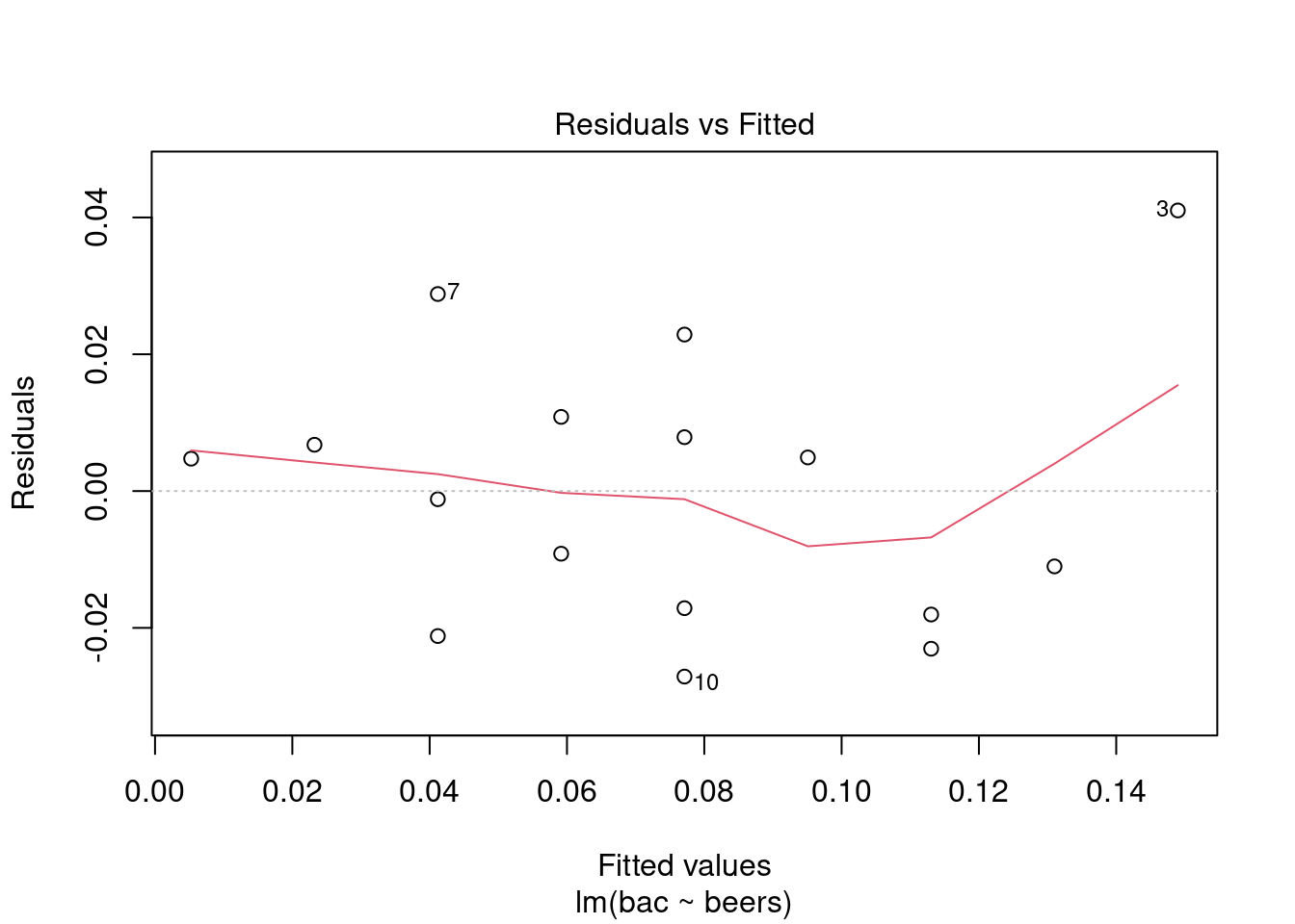
The fit is pretty good, there is one data point that is an outlier, the student that drank 9 beers.
plot(bac_mod,2)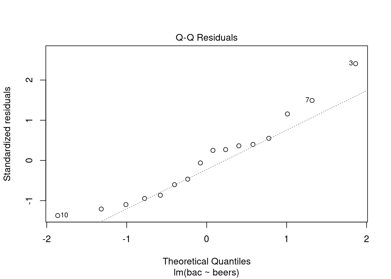
bac## # A tibble: 16 × 3
## student beers bac
## <int> <int> <dbl>
## 1 1 5 0.1
## 2 2 2 0.03
## 3 3 9 0.19
## 4 4 8 0.12
## 5 5 3 0.04
## 6 6 7 0.095
## 7 7 3 0.07
## 8 8 5 0.06
## 9 9 3 0.02
## 10 10 5 0.05
## 11 11 4 0.07
## 12 12 6 0.1
## 13 13 5 0.085
## 14 14 7 0.09
## 15 15 1 0.01
## 16 16 4 0.05The 3rd, 7th, and 10th data points stand out. This data set is too small to make any decisions about normality. It is suspect though.
plot(bac_mod,3)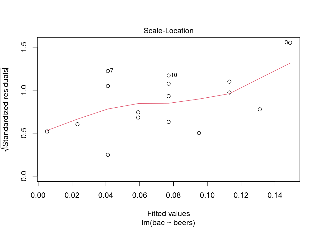
We have higher variance at the higher number of beers. Again this appears to be caused by the small number of data points and the influence of observation number 3.
plot(bac_mod,5)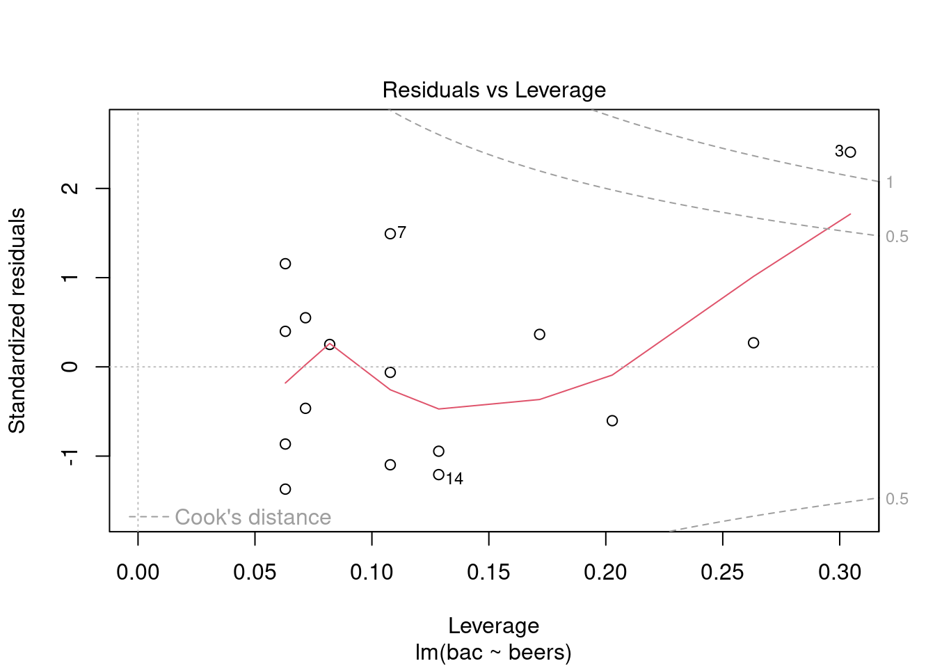
The points we’re looking for (or not looking for) are values in the upper right or lower right corners, which are outside the red dashed Cook’s distance line. These are points that would be influential in the model and removing them would likely noticeably alter the regression results. Now we see that observation 3 has extreme leverage on the model. Removing it would potentially drastically alter the model.
To learn more about measures of influence, see https://cran.r-project.org/web/packages/olsrr/vignettes/influence_measures.html
29.2.3 Problem 3
Outliers
Identify the outliers in the scatterplots shown below and determine what type of outliers they are. Explain your reasoning. The labels are off so treat the bottom row as (d), (e), and (f).
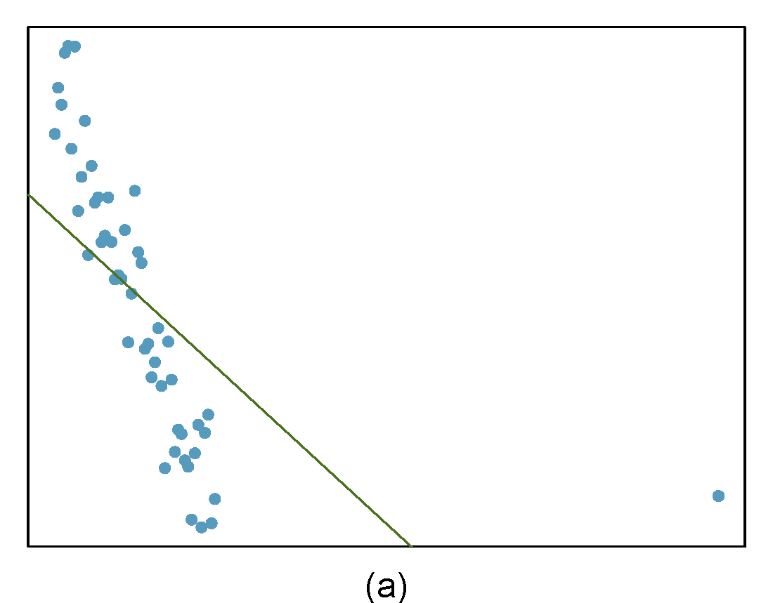
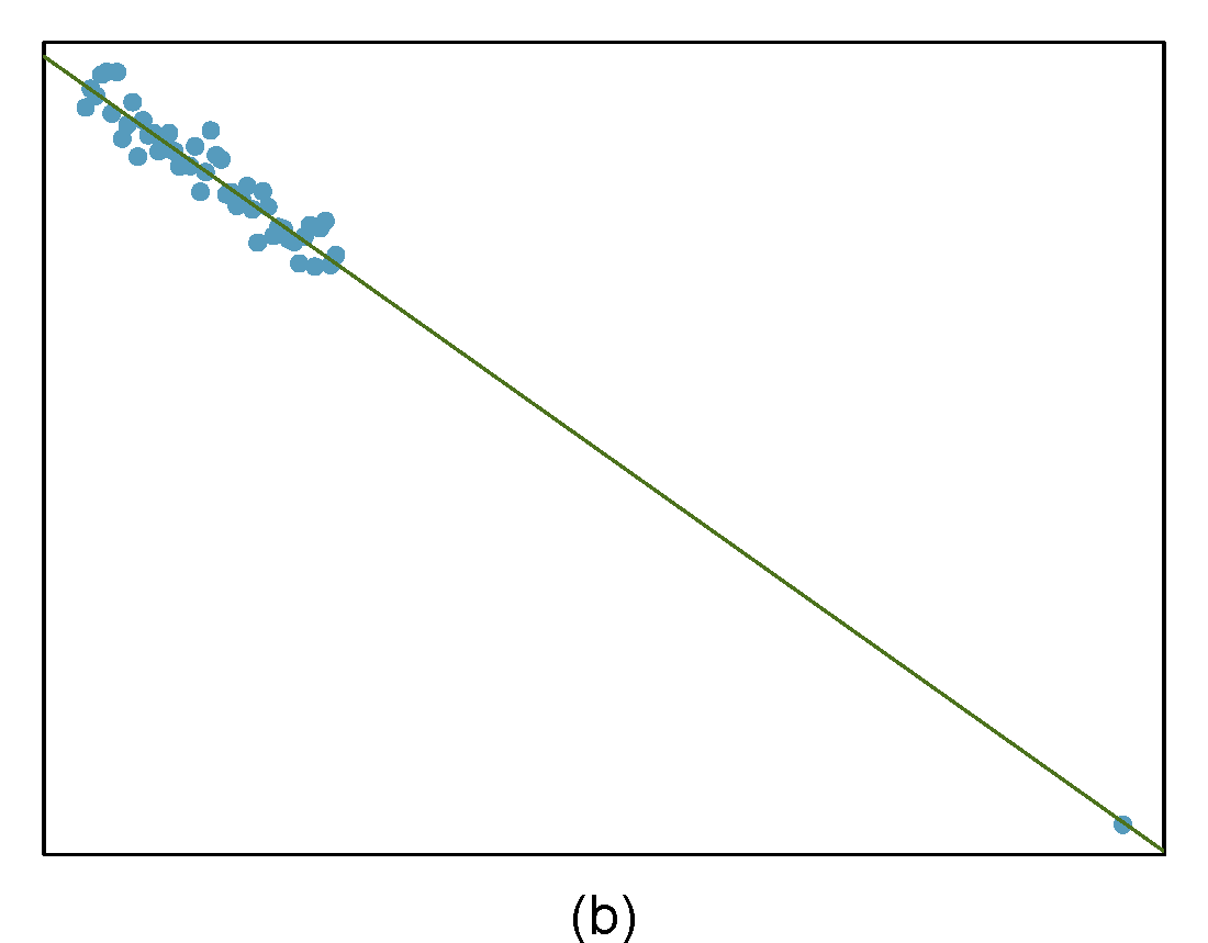
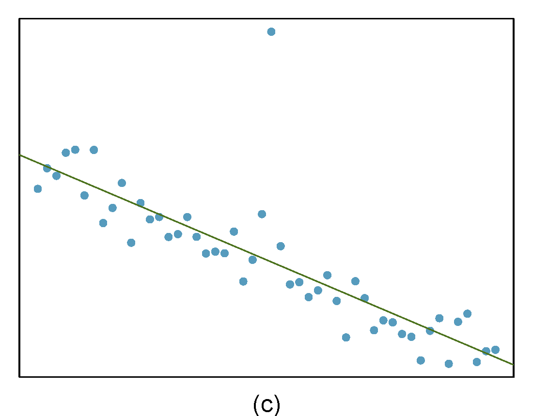
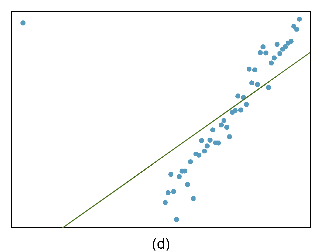
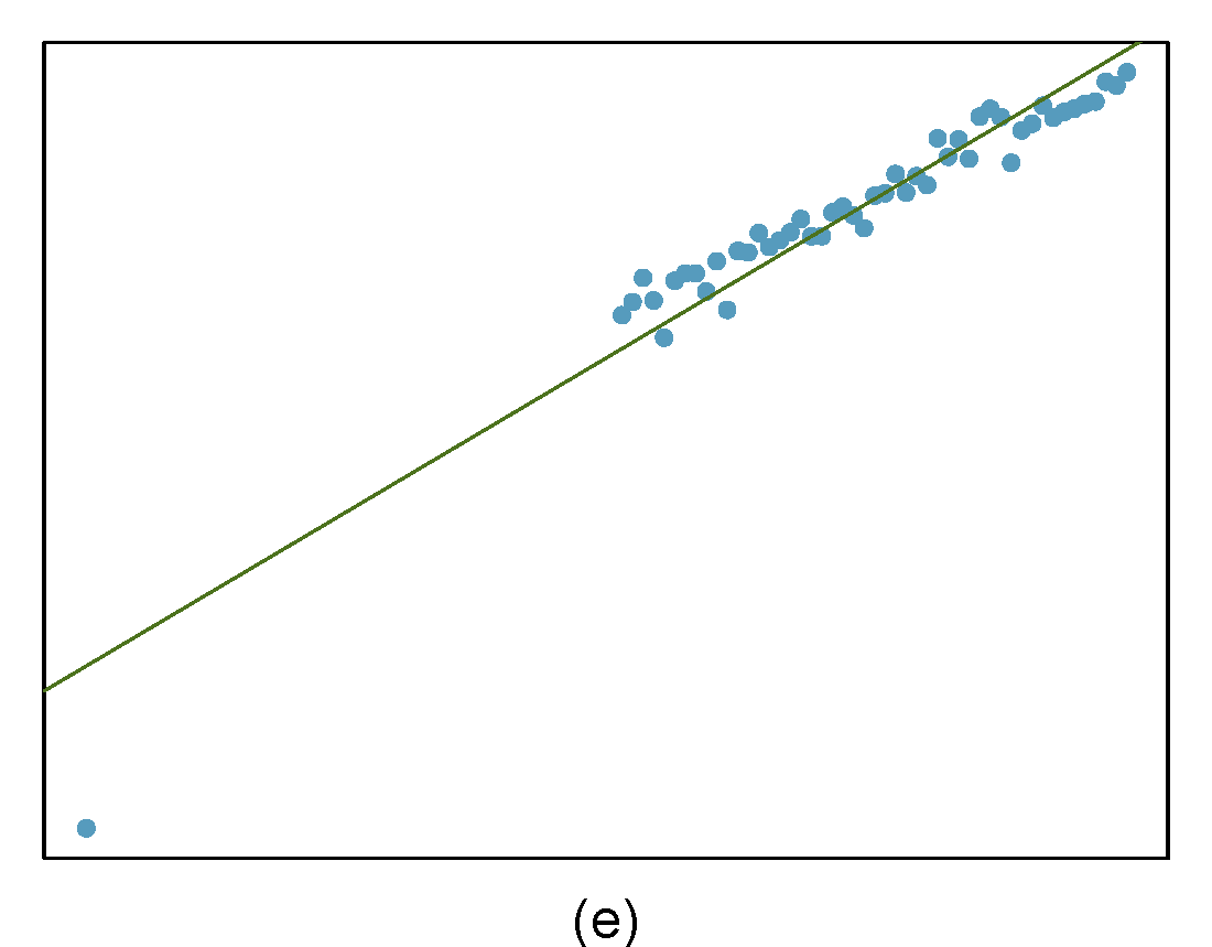
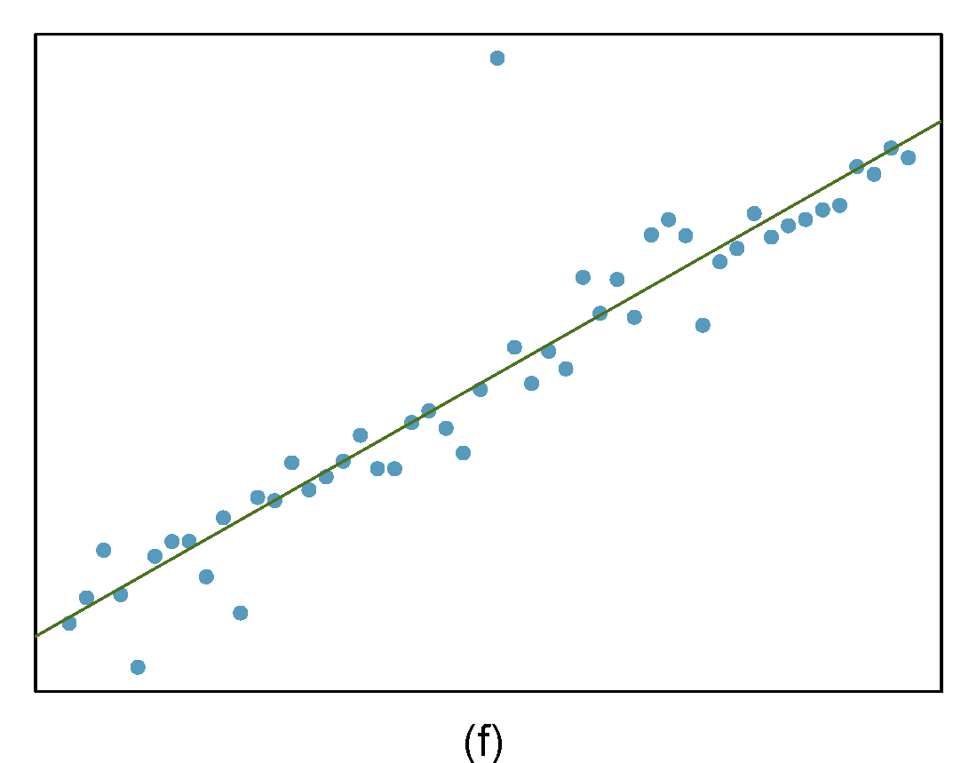
Figure 29.2: Homework problem 3.
- The outlier is located in the bottom right corner of the plot. If we were to exclude this point from the analysis, the slope of the regression line would be notably affected, which means this is a high-leverage and influential point.
- The outlier is located in the bottom right corner of the plot. It is a point with high leverage since it is horizontally away from the center of the data, but it is not influential since the regression line would change little if it was removed. It is also an outlier in the response but would have a small residual.
- The outlier is located in the center and top of the plot. Though the point is unlike the rest of the data, it is not a high-leverage point since it is not far on the x-axis from the center of the data. This also means it is not an influential point since its presence has little influence on the slope of the regression line.
- The outlier is in the upper-left corner. Since it is horizontally far from the center of the data, it is an high leverage point. Additionally, since the fit of the regression line is greatly influenced by this point, it is a influential point.
- The outlier is located in the lower-left corner. It is horizontally far from the rest of the data, so it is a high-leverage point. The regression line also would fall relatively far from this point if the fit excluded this point, meaning the outlier is influential.
- The outlier is in the upper-middle of the plot. Since it is near the horizontal center of the data, it is not a high-leverage point. This means it also will have little or no influence on the slope of the regression line.