5 Numerical Data
5.1 Objectives
Define and use properly in context all new terminology, to include: scatterplot, dot plot, mean, distribution, point estimate, weighted mean, histogram, data density, right skewed, left skewed, symmetric, mode, unimodal, bimodal, multimodal, variance, standard deviation, box plot, median, interquartile range, first quartile, third quartile, whiskers, outlier, robust estimate, transformation.
In
R, generate summary statistics for a numerical variable, including breaking down summary statistics by groups.In
R, generate appropriate graphical summaries of numerical variables.Interpret and explain output both graphically and numerically.
5.2 Homework
5.2.1 Problem 1
Mammals exploratory. Data were collected on 39 species of mammals distributed over 13 taxonomic orders. The data is in the mammals data set in the openintro package.
- Using the documentation for the
mammalsdata set, report the units for the variablebrain_wt.
?mammals
help(mammals)- Using
inspect()how many variables are numeric?
inspect(mammals)##
## categorical variables:
## name class levels n missing
## 1 species factor 62 62 0
## distribution
## 1 Africanelephant (1.6%) ...
##
## quantitative variables:
## name class min Q1 median Q3 max mean
## 1 body_wt numeric 0.005 0.600 3.3425 48.2025 6654.0 198.789984
## 2 brain_wt numeric 0.140 4.250 17.2500 166.0000 5712.0 283.134194
## 3 non_dreaming numeric 2.100 6.250 8.3500 11.0000 17.9 8.672917
## 4 dreaming numeric 0.000 0.900 1.8000 2.5500 6.6 1.972000
## 5 total_sleep numeric 2.600 8.050 10.4500 13.2000 19.9 10.532759
## 6 life_span numeric 2.000 6.625 15.1000 27.7500 100.0 19.877586
## 7 gestation numeric 12.000 35.750 79.0000 207.5000 645.0 142.353448
## 8 predation integer 1.000 2.000 3.0000 4.0000 5.0 2.870968
## 9 exposure integer 1.000 1.000 2.0000 4.0000 5.0 2.419355
## 10 danger integer 1.000 1.000 2.0000 4.0000 5.0 2.612903
## sd n missing
## 1 899.158011 62 0
## 2 930.278942 62 0
## 3 3.666452 48 14
## 4 1.442651 50 12
## 5 4.606760 58 4
## 6 18.206255 58 4
## 7 146.805039 58 4
## 8 1.476414 62 0
## 9 1.604792 62 0
## 10 1.441252 62 0- What type of variable is
danger?
It is a categorical variable indicating how much danger the mammal faces from other animals, on a scale of 1 to 5.
- Create a histogram of
total_sleepand describe the distribution.
gf_histogram(~total_sleep, data = mammals, binwidth = 2)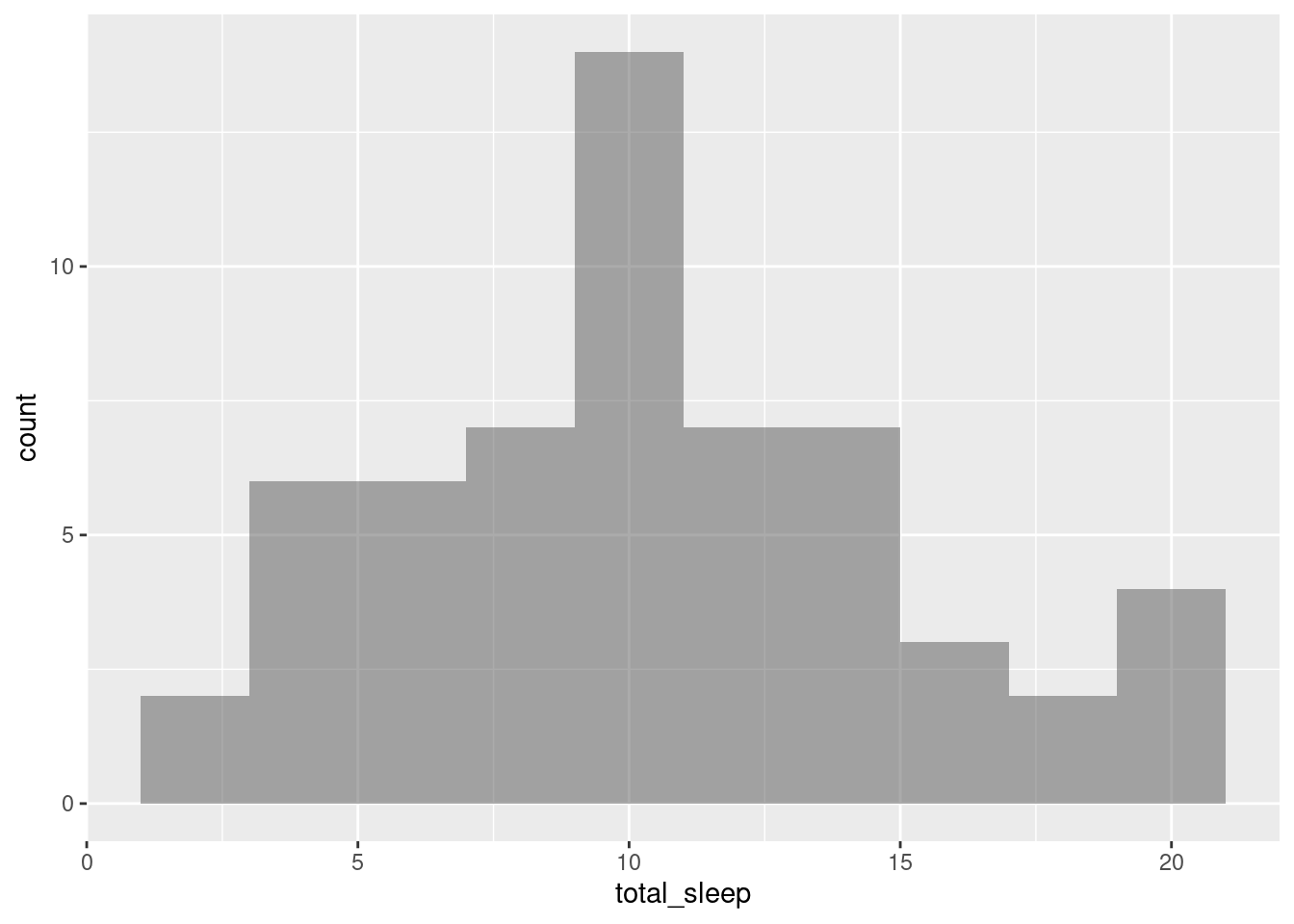
gf_dens(~total_sleep, data = mammals)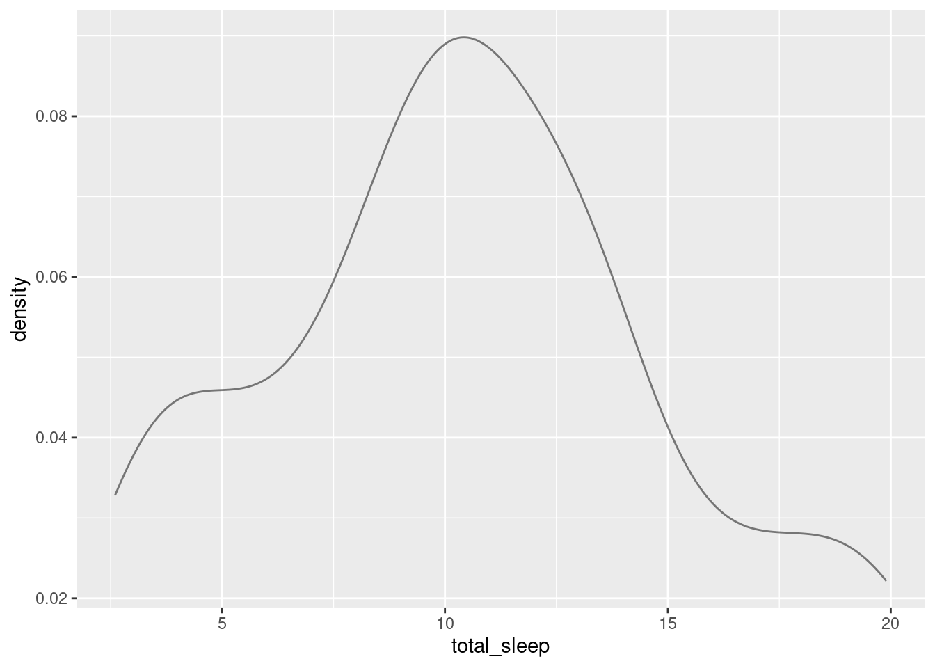
The distribution is unimodal and skewed to the right. It appears it is centered around a value of 11.
- Create a boxplot of
life_spanand describe the distribution.
gf_boxplot(~life_span, data = mammals)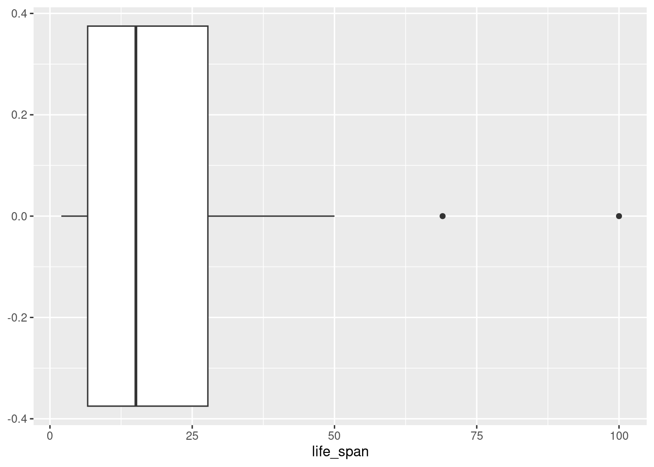
- Report the mean and median life span of a mammal.
mean(~life_span, data = mammals, na.rm = TRUE)## [1] 19.87759
median(~life_span, data = mammals, na.rm = TRUE)## [1] 15.1
favstats(~life_span, data = mammals, na.rm = TRUE)## min Q1 median Q3 max mean sd n missing
## 2 6.625 15.1 27.75 100 19.87759 18.20626 58 4- Calculate the summary statistics for
life_spanbroken down bydanger. What is the standard deviation of life span in danger outcome 5?
favstats(life_span ~ danger, data = mammals)## danger min Q1 median Q3 max mean sd n missing
## 1 1 3.0 7.700 17.60 32.500 100.0 24.20556 23.53829 18 1
## 2 2 2.3 4.500 10.40 13.000 50.0 12.92308 13.15948 13 1
## 3 3 2.0 4.175 5.35 7.875 38.6 9.43750 11.99559 8 2
## 4 4 2.6 9.775 22.10 27.000 69.0 23.11000 18.75482 10 0
## 5 5 17.0 20.000 23.60 30.000 46.0 26.95556 10.18910 9 0The standard deviation of life span in danger outcome 5 is 10.19 years.
5.2.2 Problem 2
Mammal life spans. Continue using the mammals data set.
- Create side-by-side boxplots for
life_spanbroken down byexposure. Note: you will have to changeexposureto afactor(). Report on any findings.
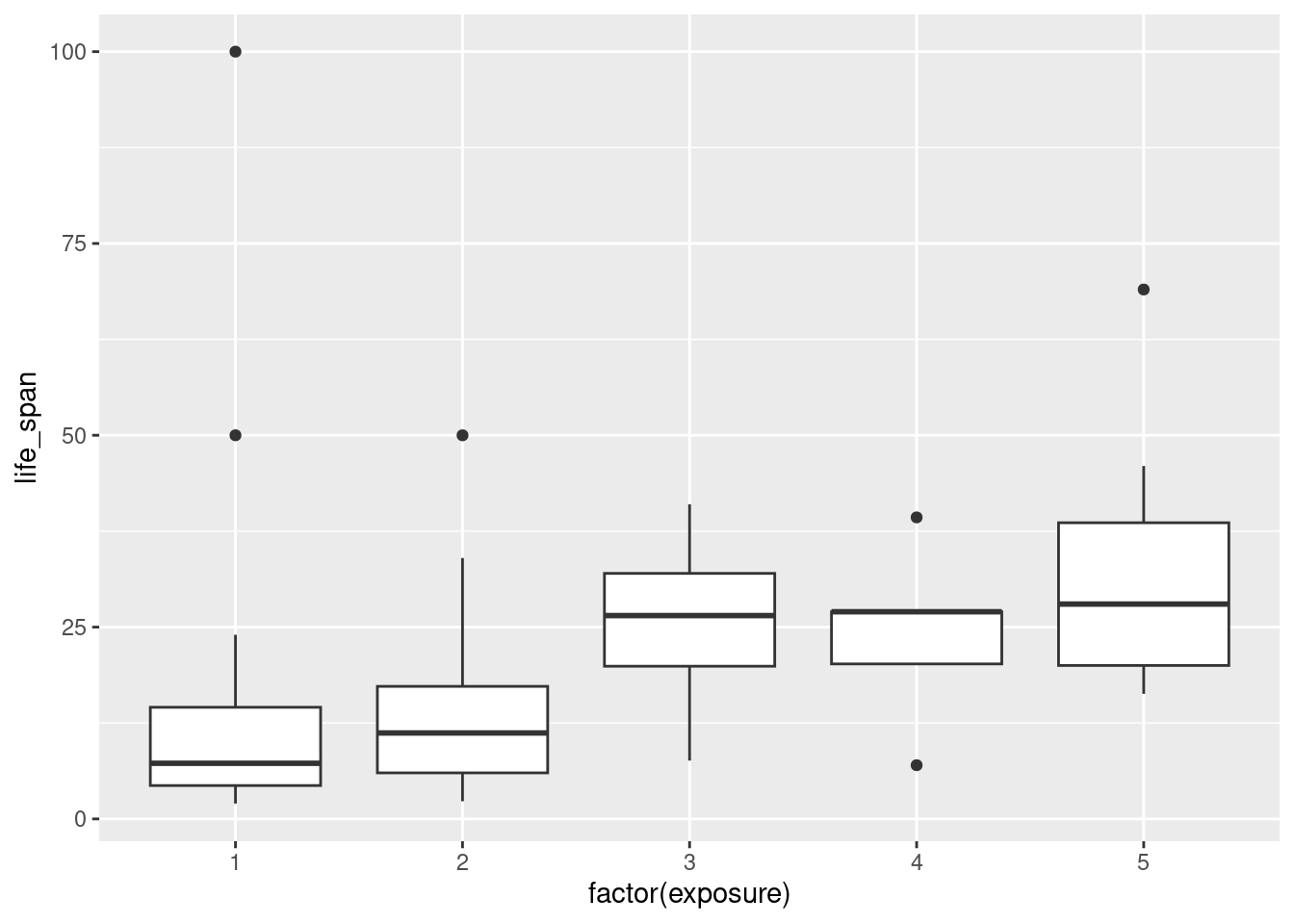
Mammals who are more exposed during sleep have a longer life span. There must be a confounding variable, such as the size of the animal or the danger variable.
- What happened to the median and third quartile in exposure group 4?
##   factor(exposure)  min    Q1 median     Q3   max     mean       sd  n missing
## 1                1  2.0  4.35   7.25 14.550 100.0 14.55000 20.98594 24       3
## 2                2  2.3  6.00  11.20 17.275  50.0 15.39167 14.55819 12       1
## 3                3  7.6 19.90  26.50 32.000  41.0 25.40000 13.84582  4       0
## 4                4  7.0 20.20  27.00 27.000  39.3 24.10000 11.78431  5       0
## 5                5 16.3 20.00  28.00 38.600  69.0 30.53077 14.98084 13       0
The median and third quartile are equal in exposure group 4. There are a large number of the observed mammals with the same life span in this group.
- Using the same variables, create faceted histograms. What are the shortcomings of this plot?
gf_histogram(~life_span|factor(exposure), data = mammals)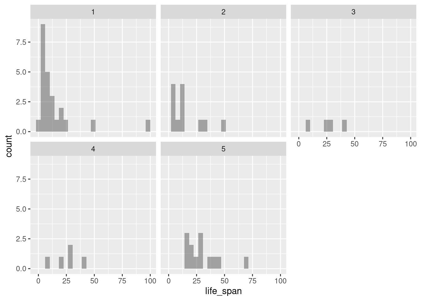
There is not enough data for each histogram; some of the histograms provide little to no information.
We can try combining this information in a single plot, coloring the plot by exposure.
gf_histogram(~life_span, color = ~factor(exposure), data = mammals)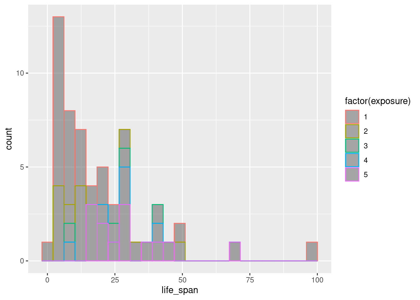
This is awful. We can also try adjusting the fill color.
gf_histogram(~life_span, fill = ~factor(exposure), data = mammals)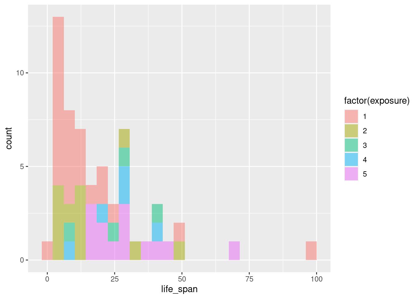
This is very difficult to look at and interpret. Let’s use density plots.
gf_dens(~life_span|factor(exposure), data = mammals)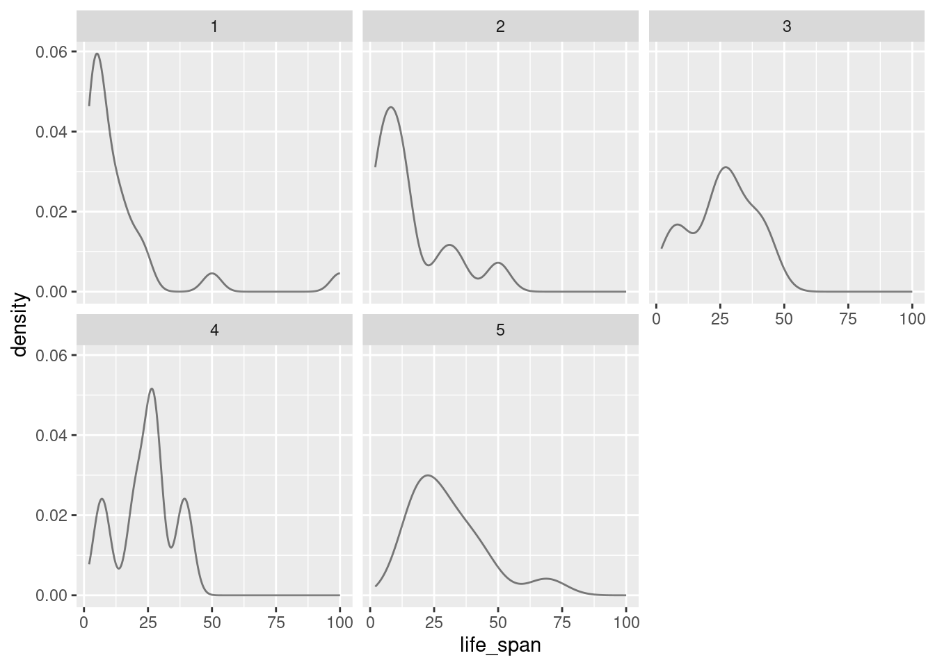
gf_dens(~life_span, color = ~factor(exposure), data = mammals)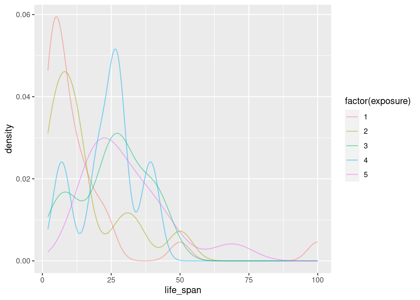
Which do you think is the best graph?
- Create a new variable
exposedthat is a factor with levelLowif exposure is1or2andHighotherwise.
mammals <- mammals %>%
  mutate(exposed = factor(ifelse((exposure == 1) | (exposure == 2),
                                 "Low", "High")))
inspect(mammals)##
## categorical variables:
## name class levels n missing
## 1 species factor 62 62 0
## 2 exposed factor 2 62 0
## distribution
## 1 Africanelephant (1.6%) ...
## 2 Low (64.5%), High (35.5%)
##
## quantitative variables:
## name class min Q1 median Q3 max mean
## 1 body_wt numeric 0.005 0.600 3.3425 48.2025 6654.0 198.789984
## 2 brain_wt numeric 0.140 4.250 17.2500 166.0000 5712.0 283.134194
## 3 non_dreaming numeric 2.100 6.250 8.3500 11.0000 17.9 8.672917
## 4 dreaming numeric 0.000 0.900 1.8000 2.5500 6.6 1.972000
## 5 total_sleep numeric 2.600 8.050 10.4500 13.2000 19.9 10.532759
## 6 life_span numeric 2.000 6.625 15.1000 27.7500 100.0 19.877586
## 7 gestation numeric 12.000 35.750 79.0000 207.5000 645.0 142.353448
## 8 predation integer 1.000 2.000 3.0000 4.0000 5.0 2.870968
## 9 exposure integer 1.000 1.000 2.0000 4.0000 5.0 2.419355
## 10 danger integer 1.000 1.000 2.0000 4.0000 5.0 2.612903
## sd n missing
## 1 899.158011 62 0
## 2 930.278942 62 0
## 3 3.666452 48 14
## 4 1.442651 50 12
## 5 4.606760 58 4
## 6 18.206255 58 4
## 7 146.805039 58 4
## 8 1.476414 62 0
## 9 1.604792 62 0
## 10 1.441252 62 0- Repeat part c) with the new
exposedvariable. Explain what you see in the plot.
gf_histogram(~life_span|exposed, data = mammals)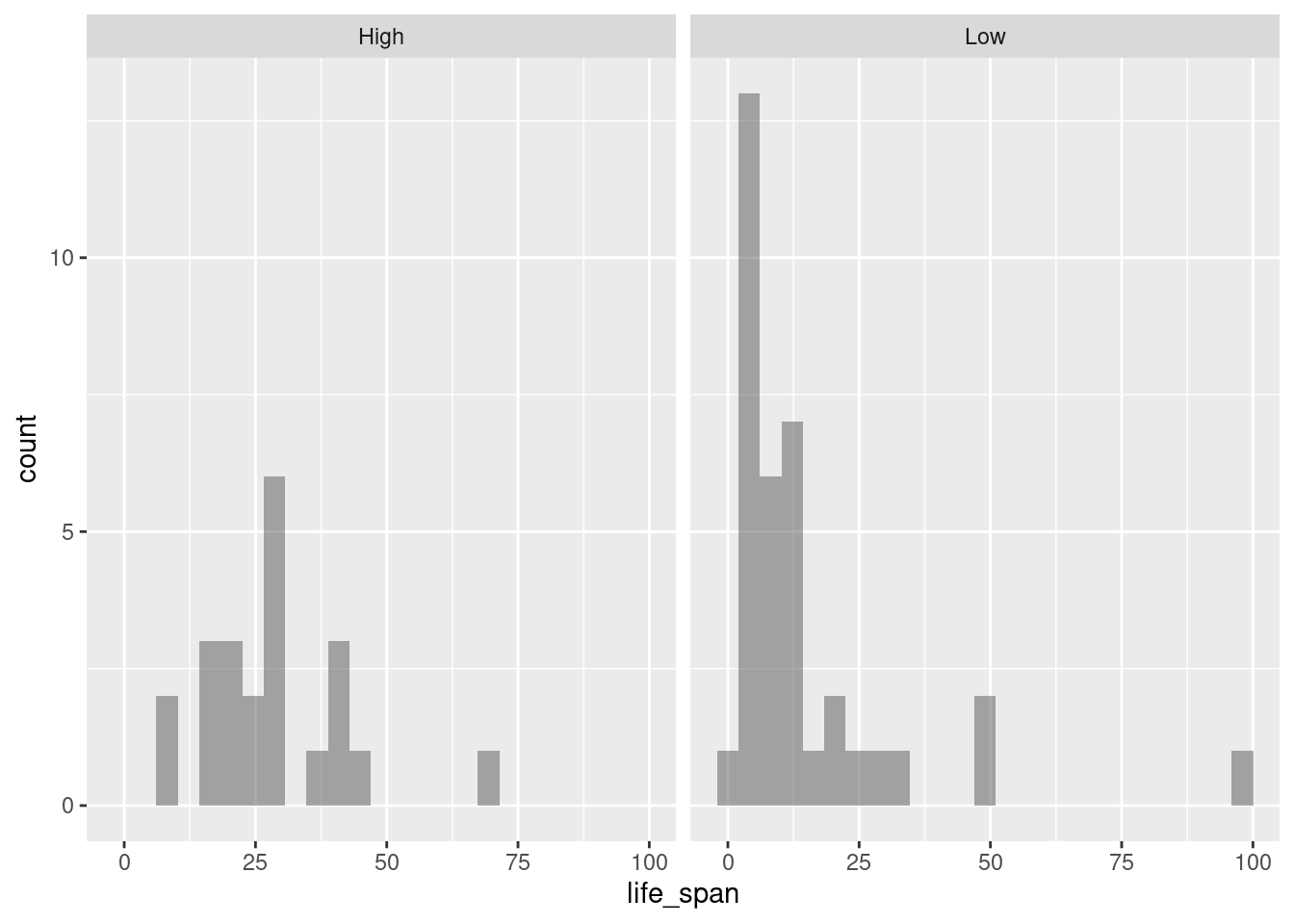
gf_dens(~life_span, color = ~exposed, data = mammals)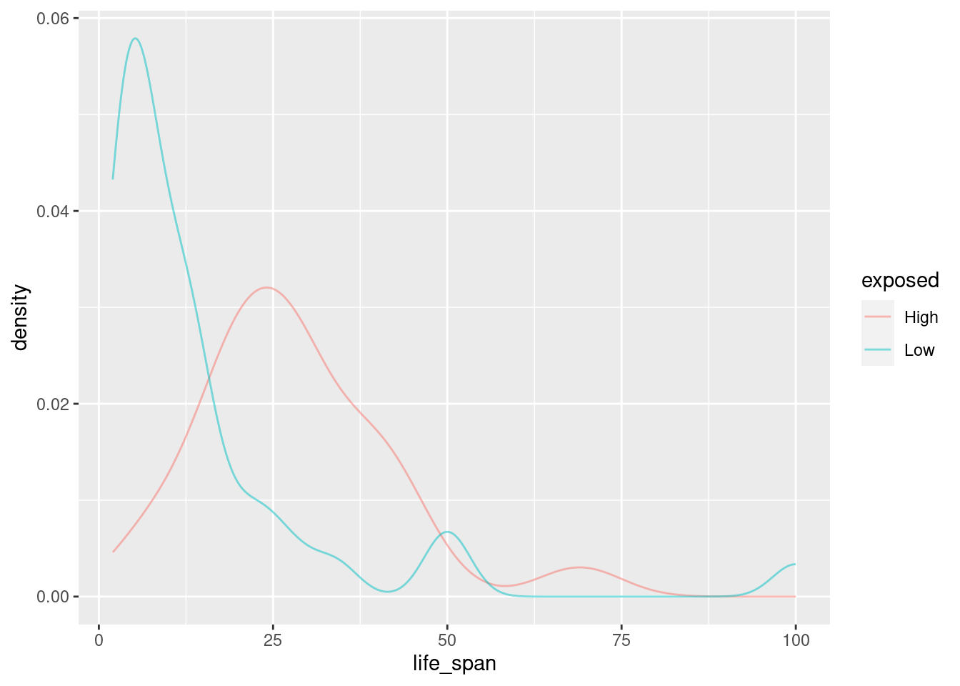
This plot is much easier to interpret. We see that higher exposure during sleep tends to result in a longer life span. It’s a lot easier to view this trend with two groups instead of five. This is a strategy we can use when we have too little data in each group.
5.2.3 Problem 3
Mammal life spans continued
- Create a scatterplot of life span versus length of gestation.
mammals %>%
  gf_point(life_span ~ gestation)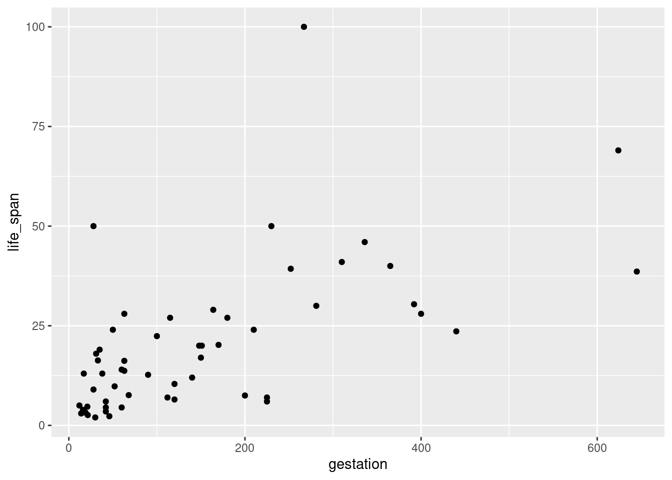
- What type of association is apparent between life span and length of gestation?
It is a weak positive association.
- What type of association would you expect to see if the axes of the plot were reversed, i.e. if we plotted length of gestation versus life span?
We would expect to see the same - a weak positive association. Since this is observational data, there is no reason to believe there is a causal relationship just by looking at the data. Switching the axis will preserve the association.
- Create the new scatterplot suggested in part c).
mammals %>%
  gf_point(gestation ~ life_span)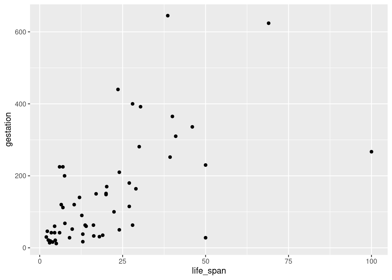
- Are life span and length of gestation independent? Explain your reasoning.
No, there is an association and it appears to be linear. If the plot looked like a “shotgun” blast, we would consider the variables to be independent. However, remember there may be confounding variables that could impact the association between these variables.