8 Probability Rules

8.1 Objectives

Differentiate between various statistical terminologies such as sample space, outcome, event, subset, intersection, union, complement, probability, mutually exclusive, exhaustive, independent, multiplication rule, permutation, and combination, and construct examples to demonstrate their proper use in context.
Apply basic probability properties and counting rules to calculate the probabilities of events in different scenarios. Interpret the calculated probabilities in context.
Explain and illustrate the basic axioms of probability.
Use R to perform calculations and simulations for determining the probabilities of events.

8.2 Probability vs Statistics

Remember this book is divided into four general blocks: data collection/summary, probability models, inference and statistical modeling/prediction. This second block on probability models is the study of stochastic (random) processes and their properties. Specifically, we will explore random experiments. As the name suggests, a random experiment is an experiment whose outcome is not predictable with exact certainty. In the statistical models we develop in the last two blocks of this book, we will use other variables to explain the variance of the outcome of interest. Any remaining variance is modeled with probability models.

Even though an outcome is determined by chance, this does not mean that we know nothing about the random experiment. Our favorite simple example is that of a coin flip. If we flip a coin, the possible outcomes are heads and tails. We don’t know for sure what outcome will occur, but we still know something about the experiment. If we assume the coin is fair, we know that each outcome is equally likely. Also, we know that if we flip the coin 100 times (independently), we are likely to see around 50 heads, and very unlikely to see 10 heads or fewer.

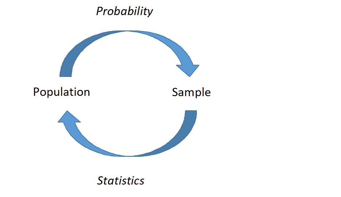
It is important to distinguish probability from inference and modeling. In probability, we consider a known random experiment, including knowing the parameters, and answer questions about what we expect to see from this random experiment. In statistics (inference and modeling), we consider data (the results of a mysterious random experiment) and infer about the underlying process. For example, suppose we have a coin and we are unsure whether this coin is fair or unfair (i.e., the parameter is unknown). We might flip it 20 times and observe it land on heads 14 times. Inferential statistics will help us answer questions about the underlying process (e.g., could this coin be unfair?).

A graphical representation of probability and statistics. In probability, we describe what we expect to happen if we know about the underlying process. In statistics, we don’t know the underlying process, and must infer based on representative samples.

This block (10 chapters or so) is devoted to the study of random experiments. First, we will explore simple experiments, counting rule problems, and conditional probability. Next, we will introduce the concept of a random variable and the properties of random variables. Following this, we will cover common distributions of discrete and continuous random variables. We will end the block on multivariate probability (joint distributions and covariance).

8.3 Basic probability terms

We will start our work with some definitions and examples.

8.3.1 Sample space

Suppose we have a random experiment. The sample space of this experiment, \(S\), is the set of all possible results of that experiment. For example, in the case of a coin flip, we could write \(S=\{H,T\}\) because the sample space has two outcomes, heads and tails. Each element of the sample space is considered an outcome. An event is a set of outcomes, a subset of the sample space.

Example:
Let R flip a coin for us and record the number of heads and tails. We will have R flip the coin twice. What is the sample space, what is an example of an outcome, and what is an example of an event?

We will load the mosaic package as it has a function rflip() that will simulate flipping a coin.

library(mosaic)

set.seed(18)
rflip(2)


Flipping 2 coins [ Prob(Heads) = 0.5 ] ...

H H

Number of Heads: 2 [Proportion Heads: 1]

The sample space is \(S=\{HH, TH, HT, TT\}\), an example of an outcome is \(HH\) which we see in the output from R, and an example of an event is two tails, \({TT}\). Another example of an event is “at least one heads”, \(\{HH,TH, HT\}\). Also, notice that \(TH\) is different from \(HT\) as an outcome; this is because those are different outcomes from flipping a coin twice.

Example of Event:
Suppose you arrive at a rental car counter and they show you a list of available vehicles, and one is picked for you at random. The sample space in this experiment is \[ S=\{\mbox{red sedan}, \mbox{blue sedan}, \mbox{red truck}, \mbox{grey truck}, \mbox{grey SUV}, \mbox{black SUV}, \mbox{blue SUV}\}. \]

Each vehicle represents a possible outcome of the experiment.

8.3.2 Union and intersection

Suppose we have two events, \(A\) and \(B\).

\(A\) is considered a subset of \(B\) if all of the outcomes of \(A\) are also contained in \(B\). This is denoted as \(A \subset B\).
The intersection of \(A\) and \(B\) is all of the outcomes contained in both \(A\) and \(B\). This is denoted as \(A \cap B\).
The union of \(A\) and \(B\) is all of the outcomes contained in either \(A\) or \(B\), or both. This is denoted as \(A \cup B\).
The complement of \(A\) is all of the outcomes not contained in \(A\). This is denoted as \(A^C\) or \(A'\).

Note: Here we are treating events as sets and the above definitions are basic set operations.

It is sometimes helpful when reading probability notation to think of Union as an or and Intersection as an and.

Example:
Consider our rental car example above. Let \(A\) be the event that a blue vehicle is selected, let \(B\) be the event that a black vehicle is selected, and let \(C\) be the event that an SUV is selected.

First, let’s list all of the outcomes of each event. \(A = \{\mbox{blue sedan},\mbox{blue SUV}\}\), \(B=\{\mbox{black SUV}\}\), and \(C= \{\mbox{grey SUV}, \mbox{black SUV}, \mbox{blue SUV}\}\).

Because all outcomes in \(B\) are contained in \(C\), we know that \(B\) is a subset of \(C\). This can be written as \(B\subset C\). Also, because \(A\) and \(B\) have no outcomes in common, \(A \cap B = \emptyset\). Note that \(\emptyset = \{ \}\) is the empty set and contains no elements.¹ Further, \(A \cup C = \{\mbox{blue sedan}, \mbox{grey SUV}, \mbox{black SUV}, \mbox{blue SUV}\}\). The complement of \(C\) is \(C'=\{\text{red sedan, red truck, grey truck}\}\).

8.4 Probability

Probability is a number assigned to an event or outcome that describes how likely it is to occur. A probability model assigns a probability to each element of the sample space. What makes a probability model is not just the values assigned to each element but the idea that this model contains all the information about the outcomes and there are no other explanatory variables involved.

A probability model can be thought of as a function that maps outcomes, or events, to a real number in the interval \([0,1]\).

8.4.1 Probability axioms

There are some basic axioms of probability you should know, although this list is not complete. Let \(S\) be the sample space of a random experiment and let \(A\) be an event where \(A\subset S\).

\(\mbox{P}(A) \geq 0\).
\(\mbox{P}(S) = 1\).

These two axioms essentially say that probability must be positive, and the probability of all outcomes must sum to one.

8.4.2 Probability properties

Let \(A\) and \(B\) be events in a random experiment. Most of the probabilities below can be proven fairly easily.

\(\mbox{P}(\emptyset)=0\).
\(\mbox{P}(A')=1-\mbox{P}(A)\). We used this in the case study.
If \(A\subset B\), then \(\mbox{P}(A)\leq \mbox{P}(B)\).
\(\mbox{P}(A\cup B) = \mbox{P}(A)+\mbox{P}(B)-\mbox{P}(A\cap B)\). This property can be generalized to more than two events. The intersection is subtracted because outcomes in both events \(A\) and \(B\) get counted twice in the first sum.
Law of Total Probability: Let \(B_1, B_2,...,B_n\) be mutually exclusive, this means disjoint or no outcomes in common, and exhaustive, this means the union of all the events labeled with a \(B\) is the sample space. Then

\[ \mbox{P}(A)=\mbox{P}(A\cap B_1)+\mbox{P}(A\cap B_2)+...+\mbox{P}(A\cap B_n) \]

A specific application of this law appears in Bayes’ Rule (more to follow in Chapter 9). It says that \(\mbox{P}(A)=\mbox{P}(A \cap B)+\mbox{P}(A \cap B')\). Essentially, it points out that \(A\) can be partitioned into two parts: 1) everything in \(A\) and \(B\) and 2) everything in \(A\) and not in \(B\).

Example:
Consider rolling a six sided die. Let event \(A\) be that a number less than five is showing on the die. Let event \(B\) be that the number is even. Then,

\[\mbox{P}(A)=\mbox{P}(A \cap B) + \mbox{P}(A \cap B')\]

\[ \mbox{P}(< 5)=\mbox{P}(<5 \cap \text{Even})+\mbox{P}(<5 \cap \text{Odd}) \]

DeMorgan’s Laws: \[ \mbox{P}((A \cup B)')=\mbox{P}(A' \cap B') \] \[ \mbox{P}((A \cap B)')=\mbox{P}(A' \cup B') \]

Exercise:
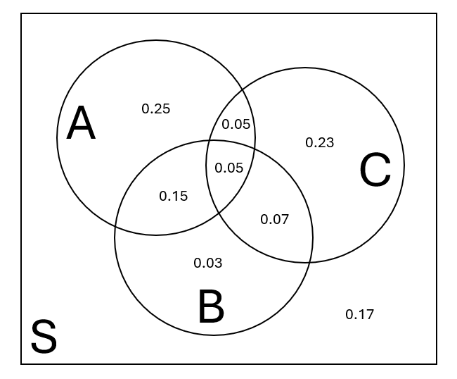
Let \(A\), \(B\), and \(C\) be events such that \(P(A)=0.5\), \(P(B)=0.3\), and \(P(C)=0.4\). Also, we know that \(P(A\cap B)=0.2\), \(P(B\cap C)=0.12\), \(P(A\cap C)=0.1\), and \(P(A\cap B\cap C)=0.05\). Find the following:

\(P(A\cup B)\)

\(P(A\cup B\cup C)\)

\(P(B'\cap C')\)

\(P(A\cup (B\cap C))\)

\(P((A\cup B\cup C)\cap (A\cap B\cap C)')\)

It can be a good idea to draw a picture to work through exercises like these. Figure 8.1 is an illustration of the above probability problem. Letters A, B, and C denote the corresponding events, represented by the entire circle in which they reside. The letter S represents the entire sample space. The numbers in the diagram represent the probability of each exclusive event. For example, the value 0.25 represents the probability of only event A (and no other events). Can you figure out where the other probability values come from?²

8.4.3 Equally likely scenarios

In some random experiments, outcomes can be defined such that each individual outcome is equally likely. In this case, probability becomes a counting problem. Let \(A\) be an event in an experiment where each outcome is equally likely. \[ \mbox{P}(A)=\frac{\mbox{Number of outcomes in A}}{\mbox{Number of outcomes in S}} \]

Example:
Suppose a family has three children, with each child being either male (M) or female (F). Assume that the likelihood of males and females are equal and independent. This is the idea that the probability of the sex of the second child does not change based on the sex of the first child. The sample space can be written as: \[ S=\{\mbox{MMM},\mbox{MMF},\mbox{MFM},\mbox{FMM},\mbox{MFF},\mbox{FMF},\mbox{FFM},\mbox{FFF}\} \] What is the probability that the family has exactly 2 female children?

This only happens in three ways: MFF, FMF, and FFM. Thus, the probability of exactly 2 females is 3/8 or 0.375.

8.4.4 Simulation with `R` (Equally likely scenarios)

The previous example above is an example of an “Equally Likely” scenario, where the sample space of a random experiment contains a list of outcomes that are equally likely. In these cases, we can sometimes use R to list out the possible outcomes and count them to determine probability. We can also use R to simulate the scenario.

Example:
Use R to simulate the family of three children where each child has the same probability of being male or female.

Instead of writing our own function, we can use rflip() in the mosaic package. We will let \(H\) stand for female.

First simulate one family.

set.seed(73)
rflip(3)


Flipping 3 coins [ Prob(Heads) = 0.5 ] ...

T T H

Number of Heads: 1 [Proportion Heads: 0.333333333333333]

In this case, we got 1 female. Next, we will use the do() function to repeat this simulation.

results <- do(10000)*rflip(3)
head(results)

  n heads tails      prop
1 3     1     2 0.3333333
2 3     3     0 1.0000000
3 3     3     0 1.0000000
4 3     3     0 1.0000000
5 3     1     2 0.3333333
6 3     1     2 0.3333333

Next, we can visualize the distribution of the number of females, heads, in Figure Figure 8.2.

results %>%
  gf_bar(~heads) %>%
  gf_theme(theme_bw()) %>%
  gf_labs(x = "Number of females", y = "Count")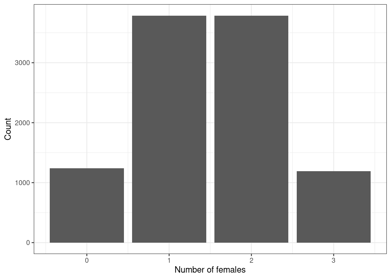

Figure 8.2: Number of females in a family of size 3.

Finally, we can estimate the probability of exactly 2 females. We need the tidyverse library.

library(tidyverse)

results %>%
  filter(heads == 2) %>%
  summarize(prob = n()/10000)

    prob
1 0.3782

Or we can use slightly different code.

results %>%
  count(heads) %>%
  mutate(prop = n/sum(n))

  heads    n   prop
1     0 1241 0.1241
2     1 3786 0.3786
3     2 3782 0.3782
4     3 1191 0.1191

This is not a bad estimate of the exact probability, 0.375.

Let’s now use an example of cards to simulate some probabilities and learn more about counting. The file Cards.csv contains the data for cards from a standard 52-card deck. There are four suits and two colors: spades and clubs are black, hearts and diamonds are red. Within each suit, there are 13 card values or ranks. These include ace, king, queen, jack, and numbers ranging from ten down to two. Let’s read in the data and summarize.

Cards <- read_csv("data/Cards.csv")
inspect(Cards)


categorical variables:  
  name     class levels  n missing
1 rank character     13 52       0
2 suit character      4 52       0
                                   distribution
1 10 (7.7%), 2 (7.7%), 3 (7.7%) ...            
2 Club (25%), Diamond (25%) ...                

quantitative variables:  
   name   class        min         Q1     median         Q3        max
1 probs numeric 0.01923077 0.01923077 0.01923077 0.01923077 0.01923077
        mean sd  n missing
1 0.01923077  0 52       0

head(Cards)

# A tibble: 6 × 3
  rank  suit   probs
  <chr> <chr>  <dbl>
1 2     Club  0.0192
2 3     Club  0.0192
3 4     Club  0.0192
4 5     Club  0.0192
5 6     Club  0.0192
6 7     Club  0.0192

We can see 4 suits, and 13 ranks, the value on the face of the card.

Example:
Suppose we draw one card out of a standard deck. Let \(A\) be the event that we draw a Club. Let \(B\) be the event that we draw a 10 or a face card (Jack, Queen, King or Ace). We can use R to define these events and find probabilities.

Let’s find all the Clubs.

Cards %>%
  filter(suit == "Club") %>%
  select(rank, suit)

# A tibble: 13 × 2
   rank  suit 
   <chr> <chr>
 1 2     Club 
 2 3     Club 
 3 4     Club 
 4 5     Club 
 5 6     Club 
 6 7     Club 
 7 8     Club 
 8 9     Club 
 9 10    Club 
10 J     Club 
11 Q     Club 
12 K     Club 
13 A     Club

So just by counting, we find the probability of drawing a Club is \(\frac{13}{52}\) or 0.25. We can also do this with simulation. This may be overkill for this example, but it gets the idea of simulation across.

Remember, ask yourself what we want R to do and what R needs to do this. Below we sample one card from “the deck” (i.e., the data set) 10,000 times.

set.seed(573)
results <- do(10000)*sample(Cards, 1)
head(results)

# A tibble: 6 × 6
  rank  suit     probs orig.id  .row .index
  <chr> <chr>    <dbl> <chr>   <int>  <dbl>
1 2     Diamond 0.0192 14          1      1
2 7     Spade   0.0192 45          1      2
3 6     Spade   0.0192 44          1      3
4 3     Heart   0.0192 28          1      4
5 5     Diamond 0.0192 17          1      5
6 10    Spade   0.0192 48          1      6

results %>%
  filter(suit == "Club") %>%
  summarize(prob = n()/10000)

# A tibble: 1 × 1
   prob
  <dbl>
1 0.240

results %>%
  count(suit) %>%
  mutate(prob = n/sum(n))

# A tibble: 4 × 3
  suit        n  prob
  <chr>   <int> <dbl>
1 Club     2405 0.240
2 Diamond  2594 0.259
3 Heart    2529 0.253
4 Spade    2472 0.247

In 10,000 samples, each suit occurs around 25% of the time, just as we’d expect.

Now let’s count the number of outcomes in \(B\).

Cards %>%
  filter(rank %in% c(10, "J", "Q", "K", "A")) %>%
  select(rank,suit)

# A tibble: 20 × 2
   rank  suit   
   <chr> <chr>  
 1 10    Club   
 2 J     Club   
 3 Q     Club   
 4 K     Club   
 5 A     Club   
 6 10    Diamond
 7 J     Diamond
 8 Q     Diamond
 9 K     Diamond
10 A     Diamond
11 10    Heart  
12 J     Heart  
13 Q     Heart  
14 K     Heart  
15 A     Heart  
16 10    Spade  
17 J     Spade  
18 Q     Spade  
19 K     Spade  
20 A     Spade

So just by counting, we find the probability of drawing a 10 or greater is \(\frac{20}{52}\) or 0.3846154.

Exercise:
Use simulation to estimate the probability of a 10 or higher (10, jack, queen, king).

We can simply examine the previously generated 10,000 samples to answer this question via simulation.

results %>%
  filter(rank %in% c(10, "J", "Q", "K", "A")) %>%
  summarize(prob = n()/10000)

# A tibble: 1 × 1
   prob
  <dbl>
1 0.382

This is close to the value of 0.385 we found with just counting the possibilities.

Notice that this code is not robust to change in the number of simulations. If we use a different number of simulations, then we have to adjust the denominator in the summarize() function. We can do this by using mutate() instead of filter().

results %>%
  mutate(face = rank %in% c(10, "J", "Q", "K", "A"))%>%
  summarize(prob = mean(face))

# A tibble: 1 × 1
   prob
  <dbl>
1 0.382

Notice in the mutate() function we are creating a new logical variable called face. This variable takes on the values of TRUE and FALSE. In the next line, we use a summarize() command with the function mean(). In R, a function that requires numeric input takes a logical variable and converts TRUE into 1 and FALSE into 0. Thus, the mean() will find the proportion of TRUE values and that is why we report it as a probability.

Next, let’s find a card that is 10 or greater and a club.

Cards %>%
  filter(rank %in% c(10, "J", "Q", "K", "A"), suit == "Club") %>%
  select(rank, suit)

# A tibble: 5 × 2
  rank  suit 
  <chr> <chr>
1 10    Club 
2 J     Club 
3 Q     Club 
4 K     Club 
5 A     Club

By counting, we find the probability of drawing a 10 or greater club is \(\frac{5}{52}\) or 0.0961538.

Exercise:
Simulate drawing one card and estimate the probability of a club that is 10 or greater.

We can again utilize the previously generated 10,000 samples.

results %>%
  mutate(face = (rank %in% c(10, "J", "Q", "K", "A")) & (suit == "Club"))%>%
  summarize(prob = mean(face))

# A tibble: 1 × 1
    prob
   <dbl>
1 0.0903

Again, our simulation results are very close to the exact value found by counting.

8.4.5 Note

We have been using R to count the number of outcomes in an event. This helped us to determine probabilities, but we limited the problems to simple ones. In our cards example, it would be more interesting for us to explore more complex events such as drawing five cards from a standard 52-card deck. Each draw of five cards is equally likely, so in order to find the probability of a flush (five cards of the same suit), we could simply list all the possible flushes and compare that to the entire sample space. Because of the large number of possible outcomes, this becomes difficult. Thus, we need to explore counting rules in more detail to help us solve more complex problems. In this course, we will limit our discussion to three basic cases. You should know that there are entire courses on discrete math and counting rules, so we will still be limited in our methods and the type of problems we can solve in this course.

8.5 Counting rules

There are three types of counting problems we will consider. In each case, we are utilizing (and possibly augmenting) the multiplication rule. All that changes is whether an element is allowed to be reused (replacement), and whether the order of selection matters. This latter question is difficult. Each case will be demonstrated with an example.

8.5.1 Rule 1: Order matters, sample with replacement

The multiplication rule is at the center of each of the three methods In this first case, we are using the idea that order matters and items can be reused. This is the multiplication rule without any modifications. Let’s use an example to help our understanding.

Example:
A license plate consists of three numeric digits (0-9) followed by three single letters (A-Z). How many possible license plates exist?

We can divide this problem into two sections. In the numeric section, we are selecting 3 objects from 10, with replacement. This means that a value can be used more than once. Clearly, order matters because a license plate starting with “432” is distinct from a license plate starting with “234”. There are \(10^3 = 1000\) ways to select the first three digits; 10 for the first, 10 for the second, and 10 for the third.

Question: Why do we multiply and not add these probabilities?³

In the alphabet section, we are selecting 3 objects from 26, where again order matters. Thus, there are \(26^3=17576\) ways to select the last three letters of the plate. Combined, there are \(10^3 \times 26^3 = 17576000\) ways to select license plates. Visually, \[ \underbrace{\underline{\quad 10 \quad }}_\text{number} \times \underbrace{\underline{\quad 10 \quad }}_\text{number} \times \underbrace{\underline{\quad 10 \quad }}_\text{number} \times \underbrace{\underline{\quad 26 \quad }}_\text{letter} \times \underbrace{\underline{\quad 26 \quad }}_\text{letter} \times \underbrace{\underline{\quad 26 \quad }}_\text{letter} = 17,576,000 \]

Next, we are going to use this new counting method to find a probability.

Exercise:
What is the probability a license plate starts with the number “8” or “0” and ends with the letter “B”?

In order to find this probability, we simply need to determine the number of ways to select a license plate starting with “8” or “0” and ending with the letter “B”. We can visually represent this event as: \[ \underbrace{\underline{\quad 2 \quad }}_\text{8 or 0} \times \underbrace{\underline{\quad 10 \quad }}_\text{number} \times \underbrace{\underline{\quad 10 \quad }}_\text{number} \times \underbrace{\underline{\quad 26 \quad }}_\text{letter} \times \underbrace{\underline{\quad 26 \quad }}_\text{letter} \times \underbrace{\underline{\quad 1 \quad }}_\text{B} = 135,200 \]

Dividing this number by the total number of possible license plates yields the probability of this event.

denom <- 10*10*10*26*26*26
num <- 2*10*10*26*26*1
num / denom

[1] 0.007692308

The probability of obtaining a license plate starting with “8” or “0” and ending with “B” is 0.0077. Simulating this would be difficult because we would need special functions to check the first number and last letter. This gets into text mining, an important subject in data science, but unfortunately we don’t have much time in this book for the topic.

8.5.2 Rule 2 (Permutation): Order Matters, Sampling Without Replacement

Consider a random experiment where we sample from a group of size \(n\), without replacement, and the outcome of the experiment depends on the order of the outcomes so order matters. The number of ways to select \(k\) objects is given by \(n(n-1)(n-2)...(n-k+1)\). This is known as a permutation and is sometimes written as \[ {}_nP_{k} = \frac{n!}{(n-k)!} \]

Recall that \(n!\) is read as “\(n\) factorial” and represents the number of ways to arrange \(n\) objects.

Example:
Twenty-five friends participate in a Halloween costume party. Three prizes are given during the party: most creative costume, scariest costume, and funniest costume. No one can win more than one prize. How many possible ways can the prizes by distributed?

There are \(k=3\) prizes to be assigned to \(n=25\) people. Once someone is selected for a prize, they are removed from the pool of eligible prize winners. In other words, we are sampling without replacement. Also, order matters because there are specific labels on the awards. For example, if Tom, Mike, and Jane win most creative, scariest and funniest costume, respectively, we have a different outcome than if Mike won creative, Jane won scariest and Tom won funniest costume. Thus, the number of ways the prizes can be distributed is given by \({}_{25}P_3 = \frac{25!}{22!} = 13,800\). A way to visualize this expression is shown as: \[ \underbrace{\underline{\quad 25 \quad }}_\text{most creative} \times \underbrace{\underline{\quad 24 \quad }}_\text{scariest} \times \underbrace{\underline{\quad 23 \quad }}_\text{funniest} = 13,800 \]

It is sometimes difficult to determine whether order matters in a problem, but in this example the named prizes were a hint that order matters. This is usually the case when there is some type of label to be attributed to individuals.

Let’s use the idea of a permutation to calculate a probability.

Exercise:
Assume that all 25 participants are equally likely to win any one of the three prizes. What is the probability that Tom doesn’t win any of them?

Just like in the previous probability calculation, we simply need to count the number of ways Tom doesn’t win any prize. In other words, we need to count the number of ways that prizes are distributed without Tom. So, remove Tom from the group of 25 eligible participants. The number of ways Tom doesn’t get a prize is \({}_{24}P_3 = \frac{24!}{21!}=12,144\). Again visually: \[ \underbrace{\underline{\quad 24 \quad }}_\text{most creative} \times \underbrace{\underline{\quad 23 \quad }}_\text{scariest} \times \underbrace{\underline{\quad 22 \quad }}_\text{funniest} = 12,144 \]

The probability Tom doesn’t get a prize is simply the second number divided by the first:

denom <- factorial(25) / factorial(25 - 3)
# Or, denom <- 25*24*23
num <- 24*23*22
num / denom

[1] 0.88

8.5.3 Rule 3 (Combination): Order Does Not Matter, Sampling Without Replacement

Consider a random experiment where we sample from a group of size \(n\), without replacement, and the outcome of the experiment does not depend on the order of the outcomes (i.e., order does not matter). The number of ways to select \(k\) objects is given by \(\frac{n!} {(n-k)!k!}\). This is known as a combination and is written as: \[ \binom{n}{k} = \frac{n!}{(n-k)!k!} \]

This is read as “\(n\) choose \(k\)”. Take a moment to compare combinations to permutations, discussed in Rule 2. The difference between these two rules is that in a combination, order no longer matters. A combination is equivalent to a permutation divided by \(k!\), the number of ways to arrange the \(k\) objects selected.

Example:
Suppose we draw five cards out of a standard 52-card deck (no jokers). How many possible five card hands are there?

In this example, order does not matter. I don’t care if I receive 3 jacks then 2 queens or 2 queens then 3 jacks. Either way, it’s the same collection of five cards in my hand. Also, we are drawing without replacement. Once a card is selected, it cannot be selected again. Thus, the number of ways to select five cards is given by: \[ \binom{52}{5} = \frac{52!}{(52-5)!5!} = 2,598,960 \]

Example:
When drawing 5 cards, what is the probability of drawing a “flush” (five cards of the same suit)?

Let’s determine how many ways to draw a flush. Recall there are four suits (clubs, hearts, diamonds and spades) and each suit has 13 ranks or values. We would like to pick five of those 13 cards and 0 of the remaining 39. Let’s consider just one of those suits (clubs): \[ \mbox{P}(\mbox{5 clubs})=\frac{\binom{13}{5}\binom{39}{0}}{\binom{52}{5}} \]

The second part of the numerator (\(\binom{39}{0}\)) isn’t necessary, since it simply represents the number of ways to select 0 objects from a group (1 way), but it helps clearly lay out the events. This brings up the point of what \(0!\) equals. By definition it is 1. This allows us to use \(0!\) in our work.

Now, we expand this to all four suits by multiplying by 4, or \(\binom{4}{1}\) since we are selecting 1 suit out of the 4: \[ \mbox{P}(\mbox{flush})=\frac{\binom{4}{1}\binom{13}{5}\binom{39}{0}}{\binom{52}{5}} \]

num<-4*choose(13,5)*1
denom<-choose(52,5)
num/denom

[1] 0.001980792

There is a probability of 0.0020 of drawing a flush in a draw of five cards from a standard 52-card deck.

Exercise:
When drawing five cards, what is the probability of drawing a “full house” (three cards of the one rank and the two of another)?

This problem uses several ideas from this chapter. We need to pick the rank of the three of a kind. Then pick 3 cards from the 4 possible. Next we pick the rank of the pair from the remaining 12 ranks. Finally pick 2 cards of that rank from the 4 possible.

\[ \mbox{P}(\mbox{full house})=\frac{\binom{13}{1}\binom{4}{3}\binom{12}{1}\binom{4}{2}}{\binom{52}{5}} \]

num<-choose(13,1)*choose(4,3)*choose(12,1)*choose(4,2)
denom<-choose(52,5)
num/denom

[1] 0.001440576

Question:
Why can’t we use \(\binom{13}{2}\) instead of \(\binom{13}{1}\binom{12}{1}\)?⁴

We have just determined that a full house has a lower probability of occurring than a flush. This is why in gambling, a flush is valued less than a full house.

8.5.4 Summary of counting rules

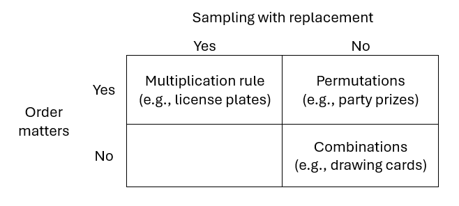
It can be difficult to remember which counting rule to use in each situation. Remember to consider whether we are sampling with or without replacement, and whether order matters. Figure 8.3 summarizes the three counting rules we discussed in this chapter.

Figure 8.3: Summary of three counting rules

We call events \(A\) and \(B\) mutually exclusive. We’ll define this term a little later in the chapter.↩︎
The easiest way to create this illustration is to start from the middle intersection piece. \(P(A\cap B\cap C)=0.05\), represented by the 0.05 at the center of the diagram. \(P(A\cap B)=0.2\), which leaves 0.15 for the rest of the \(A\cap B\) piece of the diagram. Because \(P(A\cap C)=0.1\), the remaining piece of \(A\cap C\) not yet accounted for is 0.05. Then the remaining piece of \(A\) is 0.25. Thus, \(P(A)\) can be found by summing all the pieces in the \(A\) circle, which adds up to 0.5. Make sure you can track how the rest of the diagram is appropriately labeled.↩︎
Multiplication is repeated addition, so in a sense we are adding. For this problem, every value for the first number has 10 possibilities for the second number, and for every value of the second number there are 10 possibilities for the third number. This is an “and” problem and requires multiplication.↩︎
Because this implies the order selection of the ranks does not matter. In other words, this assumes that, for example, three Kings and two fours is the same full house as 3 fours and 2 Kings. This is not true so we break the rank selection about essentially making it a permutation.↩︎