set.seed(61)
sample(1:6, size = 4, replace = TRUE)
[1] 4 2 2 1Differentiate between common discrete distributions (Uniform, Binomial, and Poisson) by identifying their parameters, assumptions, and moments. Evaluate scenarios to determine the most appropriate distribution to model various types of data.
Apply R to calculate probabilities and quantiles, and simulate random variables for common discrete distributions.
In the previous two chapters, we introduced the concept of random variables, distribution functions, and expectations. In some cases, the nature of an experiment may yield random variables with common distributions. In these cases, we can rely on easy-to-use distribution functions and built-in R functions in order to calculate probabilities and quantiles.
The first distribution we will discuss is the discrete uniform distribution. It is not a very commonly used distribution, especially compared to its continuous counterpart. A discrete random variable has the discrete uniform distribution if probability is evenly allocated to each value in the sample space. A variable with this distribution has parameters \(a\) and \(b\) representing the minimum and maximum of the sample space, respectively. (By default, that sample space is assumed to consist of integers only, but that is by no means always the case.)
Example:
Rolling a fair six-sided die is an example of the discrete uniform. Each side of the die has an equal probability.
Let \(X\) be a discrete random variable with the uniform distribution. If the sample space is consecutive integers, this distribution is denoted as \(X\sim\textsf{DUnif}(a,b)\). The pmf of \(X\) is given by: \[ f_X(x)=\left\{\begin{array}{ll}\frac{1}{b-a+1}, & x \in \{a, a+1,...,b\} \\ 0, & \mbox{otherwise} \end{array}\right. \]
The expected value of \(X\) is found by: \[ \mbox{E}(X)=\sum_{x=a}^b x\cdot\frac{1}{b-a+1}= \frac{1}{b-a+1} \cdot \sum_{x=a}^b x=\frac{1}{b-a+1}\cdot\frac{b-a+1}{2}\cdot (a+b) = \frac{a+b}{2}, \]
where the sum of consecutive integers is a common result from discrete math. Research on your own for more information.
The variance of \(X\) is found by: (derivation not included) \[ \mbox{Var}(X)=\mbox{E}[(X-\mbox{E}(X))^2]=\frac{(b-a+1)^2-1}{12} \]
Let’s summarize the discrete uniform distribution for the die:
Let \(X\) be the result of a single roll of a fair six-sided die. We will report the distribution of \(X\), the pmf, \(\mbox{E}(X)\) and \(\mbox{Var}(X)\).
The sample space of \(X\) is \(S_X=\{1,2,3,4,5,6\}\). Since each of those outcomes is equally likely, \(X\) follows the discrete uniform distribution with \(a=1\) and \(b=6\). Thus, \[ f_X(x)=\left\{\begin{array}{ll}\frac{1}{6}, & x \in \{1,2,3,4,5,6\} \\ 0, & \mbox{otherwise} \end{array}\right. \]
Finally, \(\mbox{E}(X)=\frac{1+6}{2}=3.5\). Also, \(\mbox{Var}(X)=\frac{(6-1+1)^2-1}{12}=\frac{35}{12}=2.917\).
To simulate the discrete uniform, we use sample().
Example:
To simulate rolling a die 4 times, we usesample().
set.seed(61)
sample(1:6, size = 4, replace = TRUE)[1] 4 2 2 1Let’s roll it 10,000 times and find the distribution and its moments.
results <- do(10000)*sample(1:6, size = 1, replace = TRUE)The pmf can be found using tally(). We see that each outcome has approximately the same probability, near the true value of \(1/6\).
tally(~sample, data = results, format = "percent")sample
1 2 3 4 5 6
16.40 16.46 16.83 17.15 16.92 16.24 We can find the moments by taking the mean and variance of the 10,000 simulations.
mean(~sample, data = results)[1] 3.5045var(~sample, data = results)*(10000 - 1) / 10000[1] 2.87598Notice we multiply by \(\frac{(10000-1)}{10000}\) when finding the variance. This is because the function var() is calculating a sample variance using \(n-1\) in the denominator but we need the population variance.
The binomial distribution is extremely common, and appears in many situations. In fact, we have already discussed several examples where the binomial distribution is heavily involved.
Consider an experiment involving repeated independent trials of a binary process (two outcomes), where in each trial, there is a constant probability of “success” (one of the outcomes, which is arbitrary). If the random variable \(X\) represents the number of successes out of \(n\) independent trials, then \(X\) is said to follow the binomial distribution with parameters \(n\) (the number of trials) and \(p\) (the probability of a success in each trial).
The pmf of \(X\) is given by: \[ f_X(x)=\mbox{P}(X=x)={n\choose{x}}p^x(1-p)^{n-x} \]
for \(x \in \{0,1,...,n\}\) and 0 otherwise.
Let’s take a moment to dissect this pmf. We are looking for the probability of obtaining \(x\) successes out of \(n\) trials. The \(p^x\) represents the probability of \(x\) successes, using the multiplication rule because of the independence assumption. The term \((1-p)^{n-x}\) represents the probability of the remainder of the trials as failures. Finally, the \(n\choose x\) term represents the number of ways to obtain \(x\) successes out of \(n\) trials. For example, there are three ways to obtain 1 success out of 3 trials (one success followed by two failures; one failure, one success and then one failure; or two failures followed by a success).
The expected value of a binomially distributed random variable is given by \(\mbox{E}(X)=np\) and the variance is given by \(\mbox{Var}(X)=np(1-p)\).
Example:
Let \(X\) be the number of heads out of 20 independent flips of a fair coin. Note that this is a binomial because the trials are independent and the probability of success, in this case a heads, is constant, and there are two outcomes. Find the distribution, mean and variance of \(X\). Find \(\mbox{P}(X=8)\). Find \(\mbox{P}(X\leq 8)\).
\(X\) has the binomial distribution with \(n=20\) and \(p=0.5\). The pmf is given by: \[ f_X(x)=\mbox{P}(X=x)={20 \choose x}0.5^x (1-0.5)^{20-x} \]
Also, \(\mbox{E}(X)=20*0.5=10\) and \(\mbox{Var}(X)=20*0.5*0.5=5\).
To find \(\mbox{P}(X=8)\), we can simply use the pmf: \[ \mbox{P}(X=8)=f_X(8)={20\choose 8}0.5^8 (1-0.5)^{12} \]
choose(20, 8)*0.5^8*(1 - 0.5)^12[1] 0.1201344To find \(\mbox{P}(X\leq 8)\), we would need to find the cumulative probability: \[ \mbox{P}(X\leq 8)=\sum_{x=0}^8 {20\choose 8}0.5^x (1-0.5)^{20-x} \]
x <- 0:8
sum(choose(20, x)*0.5^x*(1 - 0.5)^(20 - x))
[1] 0.2517223One of the advantages of using named distributions is that most software packages have built-in functions that compute probabilities and quantiles for common named distributions. Over the course of this chapter, you will notice that each named distribution is treated similarly in R. There are four main functions tied to each distribution. For the binomial distribution, these are dbinom(), pbinom(), qbinom(), and rbinom().
dbinom(): This function is equivalent to the probability mass function for discrete random variables. We use this to find \(\mbox{P}(X=x)\) when \(X\sim \textsf{Binom}(n,p)\). This function takes three inputs: x (the value of the random variable), size (the number of trials, \(n\)), and prob (the probability of success, \(p\)). So, \[
\mbox{P}(X=x)={n\choose{x}}p^x(1-p)^{n-x}=\textsf{dbinom(x,n,p)}
\]
pbinom(): This function is equivalent to the cumulative distribution function. We use this to find \(\mbox{P}(X\leq x)\) when \(X\sim \textsf{Binom}(n,p)\). This function takes the same inputs as dbinom() but returns the cumulative probability: \[
\mbox{P}(X\leq x)=\sum_{k=0}^x{n\choose{k}}p^k(1-p)^{n-k}=\textsf{pbinom(x,n,p)}
\]
qbinom(): This is the inverse of the cumulative distribution function and will return a percentile. This function has three inputs: p (a probability), size and prob. It returns the smallest value \(x\) such that \(\mbox{P}(X\leq x) \geq p\).
rbinom(): This function is used to randomly generate values from the binomial distribution. It takes three inputs: n (the number of values to generate), size and prob. It returns a vector containing the randomly generated values.
To learn more about these functions, type ? followed by the function name in the console or use the help() function.
Exercise:
Use the built-in functions for the binomial distribution to plot the pmf of \(X\) from the previous coin flip example. Also, use the built-in functions to compute the probabilities from the example.
Figure 12.1 displays the pmf of a binomial distribution, where \(X\) is the number of heads out of 20 independent flips of a fair coin \((p=0.5)\). The gf_dist() function helps us plot distributions by specifying the distribution name (or an abbreviation of it) and its parameters.
gf_dist("binom", size = 20, prob = 0.5) %>%
  gf_theme(theme_bw()) %>%
  gf_labs(x = "X", y = "P(X = x)")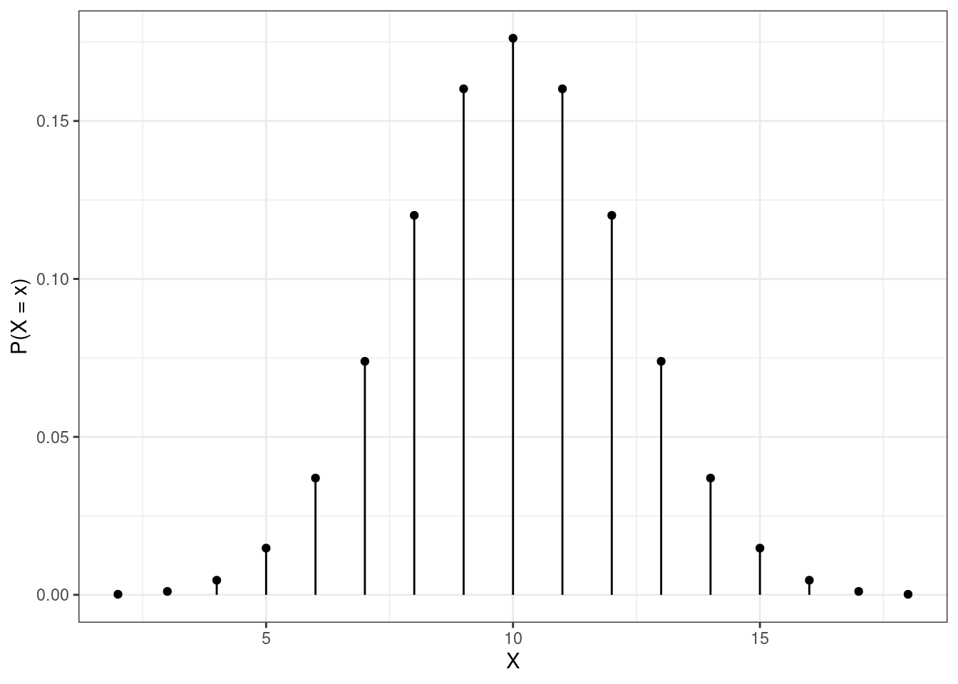
We use dbinom() to calculate probabilities of exact values such as \(P(X = 8)\). We use pbinom() to calculate cumulative probabilities such as \(P(X\leq 8)\). We can also find \(P(X\leq 8)\) by using dbinom() to calculate \(P(X=0), P(X=1), ..., P(X=8)\) and then sum them up.
###P(X = 8)
dbinom(8, 20, 0.5)
[1] 0.1201344###P(X <= 8)
pbinom(8, 20, 0.5)[1] 0.2517223## or
sum(dbinom(0:8, 20, 0.5))[1] 0.2517223The Poisson distribution is very common when considering count or arrival data. Consider a random process where events occur according to some rate over time (think arrivals to a retail register). Often, these events are modeled with the Poisson process. The Poisson process assumes a consistent rate of arrival and a memoryless arrival process (the time until the next arrival is independent of time since the last arrival). If we assume a particular process is a Poisson process, then there are two random variables that take common named distributions. The number of arrivals in a specified amount of time follows the Poisson distribution. Also, the amount of time until the next arrival follows the exponential distribution. We will defer discussion of the exponential distribution until the next chapter. What is random in the Poisson is the number of occurrences while the interval is fixed. That is why it is a discrete distribution. The parameter \(\lambda\) is the average number of occurrences in the specific interval. Note that the interval must be the same as is specified in the random variable.
Let \(X\) be the number of arrivals in a length of time, \(T\), where arrivals occur according to a Poisson process with an average of \(\lambda\) arrivals in length of time \(T\). Then \(X\) follows a Poisson distribution with parameter \(\lambda\): \[ X\sim \textsf{Poisson}(\lambda) \]
The pmf of \(X\) is given by: \[ f_X(x)=\mbox{P}(X=x)=\frac{\lambda^xe^{-\lambda}}{x!}, \hspace{0.5cm} x=0,1,2,... \]
One unique feature of the Poisson distribution is that \(\mbox{E}(X)=\mbox{Var}(X)=\lambda\).
Example:
Suppose fleet vehicles arrive to a maintenance garage at an average rate of 0.4 per day. Let’s assume that these vehicles arrive according to a Poisson process. Let \(X\) be the number of vehicles that arrive to the garage in a week (7 days). Notice that the time interval has changed! What is the random variable \(X\)? What is the distribution (with parameter) of \(X\). What are \(\mbox{E}(X)\) and \(\mbox{Var}(X)\)? Find \(\mbox{P}(X=0)\), \(\mbox{P}(X\leq 6)\), \(\mbox{P}(X \geq 2)\), and \(\mbox{P}(2 \leq X \leq 8)\). Also, find the median of \(X\), and the 95th percentile of \(X\) (the value of \(x\) such that \(\mbox{P}(X\leq x)\geq 0.95\)). Further, plot the pmf of \(X\).
Since vehicles arrive according to a Poisson process, the probability question leads us to define the random variable \(X\) as the number of vehicles that arrive in a week.
We know that \(X\sim \textsf{Poisson}(\lambda=0.4*7=2.8)\). Thus, \(\mbox{E}(X)=\mbox{Var}(X)=2.8\).
The parameter is the average number of vehicles that arrive in a week. Now, we can write the pmf of \(X\) and calculate probabilities of interest:
\[ \mbox{P}(X=0)=\frac{2.8^0 e^{-2.8}}{0!}=e^{-2.8}=0.061 \]
Alternatively, we can use the built-in R functions for the Poisson distribution.
Now, let’s calculate \(\mbox{P}(X=0)\), \(\mbox{P}(X\leq 6)\), \(\mbox{P}(X \geq 2)\), and \(\mbox{P}(2 \leq X \leq 8)\).
##P(X = 0)
dpois(0, lambda = 2.8)
[1] 0.06081006##P(X <= 6)
ppois(6, lambda = 2.8)[1] 0.9755894## or
sum(dpois(0:6, 2.8))[1] 0.9755894##P(X >= 2) = 1 - P(X < 2) = 1 - P(X <= 1)
1 - ppois(1, 2.8)[1] 0.7689218## or
sum(dpois(2:1000, 2.8))[1] 0.7689218Note that when considering \(\mbox{P}(X\geq 2)\), we recognize that this is equivalent to \(1-\mbox{P}(X\leq 1)\). We can use ppois() to find this probability or sum the probabilities for \(X\geq 2\).
When considering \(\mbox{P}(2\leq X \leq 8)\), we need to make sure we formulate this correctly. Below are two possible methods:
##P(2 <= X <= 8) = P(X <= 8) - P(X <= 1)
ppois(8, lambda = 2.8) - ppois(1, lambda = 2.8)
[1] 0.766489## or
sum(dpois(2:8, lambda = 2.8))[1] 0.766489The median is \(x\) such that \(P(X\leq x)=0.5\). To find the median and the 95th percentiles, we use qpois:
qpois(0.5, lambda = 2.8)[1] 3qpois(0.95, lambda = 2.8)[1] 6Figure 12.2 is a plot of the pmf of a Poisson random variable.
gf_dist("pois", lambda = 2.8) %>%
  gf_theme(theme_bw()) %>%
  gf_labs(x = "X", y = "P(X = x)")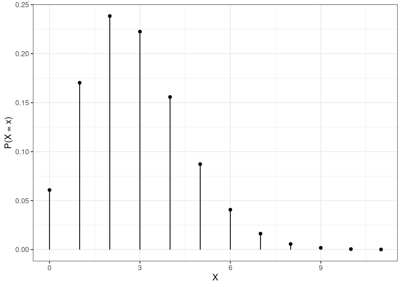
We can also simulated Poisson random variables from this distribution using the rpois() function. Suppose we want to simulate 5 random values from this Poisson distribution with a rate of \(\lambda = 2.8\).
set.seed(1)
rpois(5, lambda = 2.8)
[1] 2 2 3 5 1Remember, \(X\) is the number of vehicles that arrive to the maintenance garage in a week. These simulated values represent a week where two vehicles arrived, then another week where two vehicles arrived, followed by a week with three vehicles, then five, and then one vehicle.
There are several other named discrete distributions such as:
Bernoulli - utilized for single trial experiments with binary outcomes
Geometric - models the number of trials until the first success (often used with reliability testing)
Negative binomial - number of trials until a specified number of successes (models counts that occur in nature; used in epidemiology)
Hypergeometric - used for finding the number of successes in draws without replacement (e.g., number of red chips from a bag of red and blue chips)
Multinomial - similar to the binomial distribution, but allows for more than two outcomes (often used with Likert scale data or in polling)
We leave the details of additional discrete distributions to interested learners.