integrate(function(x)2*x, 0, 1)1 with absolute error < 1.1e-14Differentiate between various statistical terminologies such as probability density function (pdf) and cumulative distribution function (cdf) for continuous random variables, and construct examples to demonstrate their proper use in context.
For a given continuous random variable, derive and interpret the probability density function (pdf) and apply this function to calculate the probabilities of various events.
Calculate and interpret the moments, such as the expected value/mean and variance, of a continuous random variable.
In the last chapter, we introduced random variables, and explored examples and behavior of discrete random variables. In this chapter, we will shift our focus to continuous random variables, their properties, their distribution functions, and how they differ from discrete random variables.
Recall that a continuous random variable has a domain that is a continuous interval (or possibly a group of intervals). For example, let \(Y\) be the random variable corresponding to the height of a randomly selected individual. While our measurement will necessitate “discretizing” height to some degree, technically, height is a continuous random variable since a person could measure 67.3 inches or 67.4 inches or anything in between.
So how do we describe the randomness of continuous random variables? In the case of discrete random variables, the probability mass function (pmf) and the cumulative distribution function (cdf) are used to describe randomness. However, recall that the pmf is a function that returns the probability that the random variable takes the inputted value. Due to the nature of continuous random variables, the probability that a continuous random variable takes on any one individual value is technically 0. Thus, a pmf cannot apply to a continuous random variable.
Rather, we describe the randomness of continuous random variables with the probability density function (pdf) and the cumulative distribution function (cdf). Note that the cdf has the same interpretation and application as in the discrete case.
Let \(X\) be a continuous random variable. The probability density function (pdf) of \(X\), given by \(f_X(x)\) is a function that describes the behavior of \(X\). It is important to note that in the continuous case, \(f_X(x)\neq \mbox{P}(X=x)\), because the probability of \(X\) taking any one individual value is 0.
The pdf is a function. The input of a pdf is any real number. The output is known as the density. The pdf has three main properties:
\(f_X(x)\geq 0\)
\(\int_{S_X} f_X(x)\mbox{d}x = 1\)
\(\mbox{P}(X\in A)=\int_{x\in A} f_X(x)\mbox{d}x\), or another way to write this \(\mbox{P}(a \leq X \leq b)=\int_{a}^{b} f_X(x)\mbox{d}x\)
Properties 2) and 3) imply that the area underneath a pdf represents probability. Property 1) says the pdf is a non-negative function, it cannot have negative values.
The cumulative distribution function (cdf) of a continuous random variable has the same interpretation as it does for a discrete random variable. It is a function. The input of a cdf is any real number, and the output is the probability that the random variable takes a value less than or equal to the inputted value. It is denoted as \(F\) and is given by: \[ F_X(x)=\mbox{P}(X\leq x)=\int_{-\infty}^x f_x(t) \mbox{d}t \]
Example:
Let \(X\) be a continuous random variable with \(f_X(x)=2x\) where \(0 \leq x \leq 1\). Verify that \(f\) is a valid pdf. Find the cdf of \(X\). Also, find the following probabilities: \(\mbox{P}(X<0.5)\), \(\mbox{P}(X>0.5)\), and \(\mbox{P}(0.1\leq X < 0.75)\). Finally, find the median of \(X\).
To verify that \(f\) is a valid pdf, we simply note that \(f_X(x) \geq 0\) on the range \(0 \leq x \leq 1\). Also, we note that \(\int_0^1 2x \mbox{d}x = x^2\bigg|_0^1 = 1\). That is, the area under the pdf curve is one. We are essentially taking a sum over the sample space of \(X\), but \(X\) is a continuous random variable so we must integration to find the area under the curve.
Using R, we find
integrate(function(x)2*x, 0, 1)1 with absolute error < 1.1e-14We can also use the mosaicCalc package to find the anti-derivative, but we leave that method to the interested learner. If the package is not installed, you can use the Packages tab in RStudio or type install.packages("mosaicCalc") at the command prompt. Then, load the library.
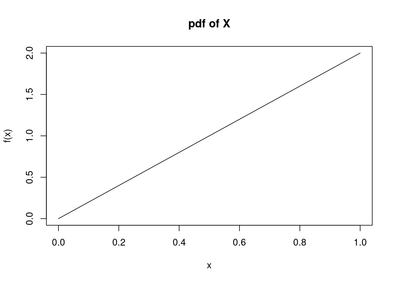
Graphically, the pdf is displayed in Figure 11.1:
Probabilities are found by integrating the pdf. The interested learner can also derive and use the cdf, but we continue to de-emphasize the cdf in this book.
We first want to find \(P(X < 0.5)\). See Figure 11.2 for an illustration of the area under the curve, the probability of interest.
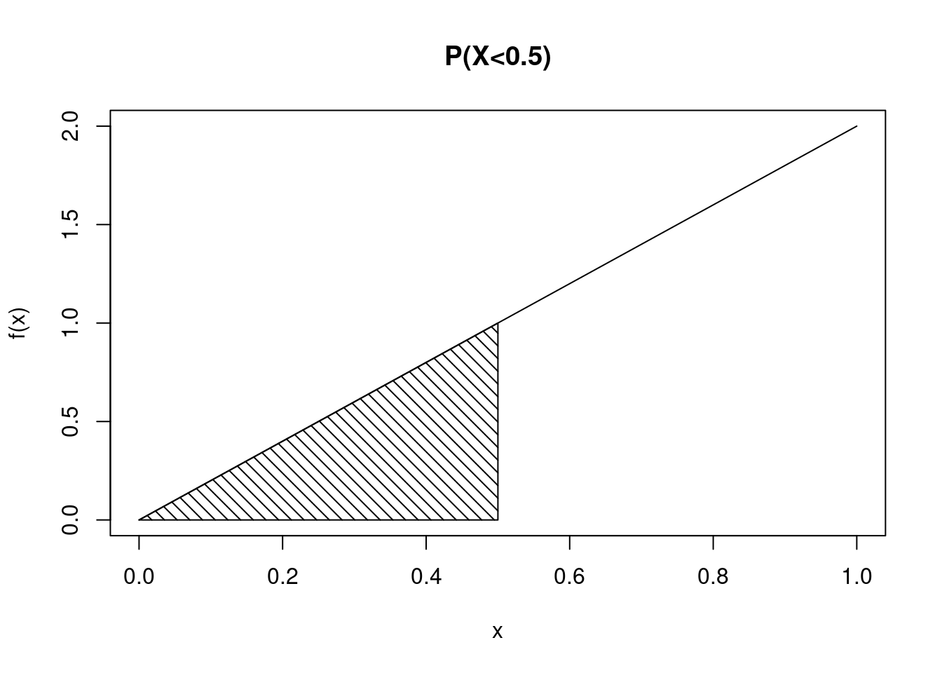
One way to find the probability is to integrate \(f_X(x)\) from 0 to 0.5.
\[\mbox{P}(X < 0.5)=\mbox{P}(X\leq 0.5) = \int_{0}^{0.5}2x = x^2\big|_{0}^{0.5} = 0.5^2 = 0.25\]
Rather than performing this integral by hand, we can also use the integrate() function in R.
integrate(function(x) 2*x, lower = 0, upper = 0.5)0.25 with absolute error < 2.8e-15Next, let’s find \(P(X > 0.5)\). See Figure 11.3 for an illustration of the region of interest. We can find this value using some algebra skills or using integrate().
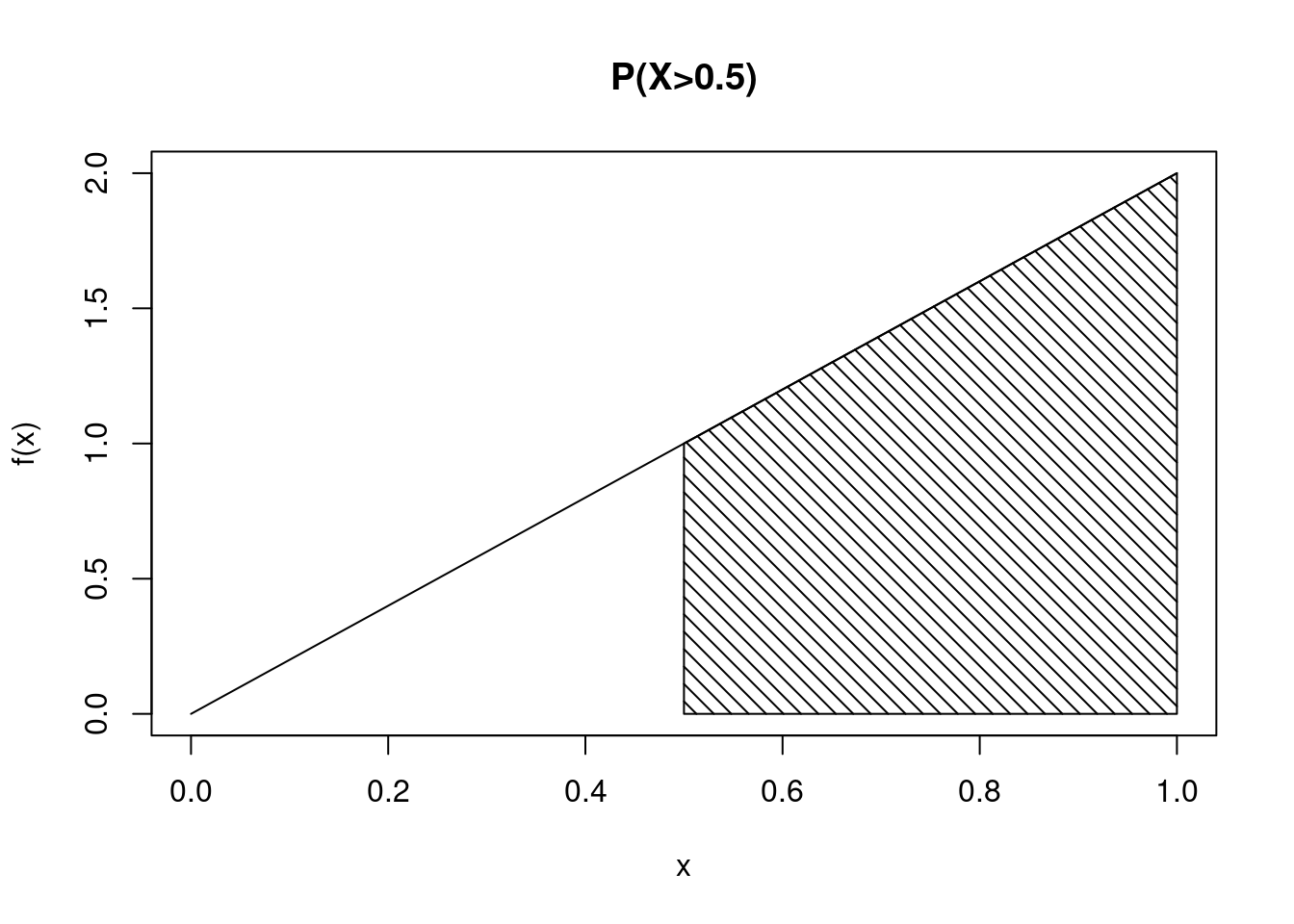
We can find the value mathematically: \(\mbox{P}(X > 0.5) = 1-\mbox{P}(X\leq 0.5)=1-0.25 = 0.75\)
Or by using R:
integrate(function(x) 2*x, lower = 0.5, upper = 1)0.75 with absolute error < 8.3e-15Finally, let’s find \(\mbox{P}(0.1\leq X < 0.75)\). See Figure 11.4 for an illustration of this region under the curve.
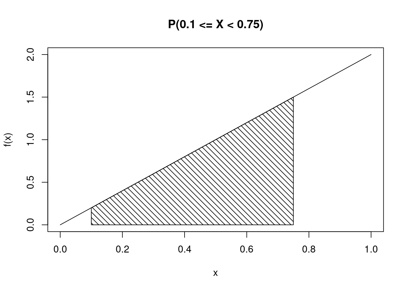
Again, we can find the value mathematically: \(\mbox{P}(0.1\leq X < 0.75) = \int_{0.1}^{0.75}2x dx = 0.75^2 - 0.1^2 = 0.5525\)
Or by using R:
integrate(function(x) 2*x, lower = 0.1, upper = 0.75)0.5525 with absolute error < 6.1e-15Notice for a continuous random variable, we are loose with the use of the = sign. This is because for a continuous random variable \(\mbox{P}(X=x)=0\). Do not get sloppy when working with discrete random variables.
The median of \(X\) is the value \(x\) such that \(\mbox{P}(X\leq x)=0.5\). One way to find this is to set the cdf equal to the quantile of interest, 0.5.1 But we don’t need the cdf if we perform a simulation and then calculate the median; we’ll do this next.
Like with discrete random variables, we can get an estimate of the pdf via simulation. However, simulating continuous random variables take a little more work.
Let’s start by generating random samples from \(X\). We can do this using a method called rejection sampling. Rejection sampling involves generating candidate points from a proposal distribution (usually a uniform distribution, with values between 0 and 1) and accepting them with a certain probability that ensures the desired distribution. To determine the probability of rejection, we essentially check whether a second random number \(u\) is less than or equal to a specific function value. For example, if we want values where \(y = 2x\), we’ll check whether \(u\leq 2x\).
Our candidate points will be generated from a uniform distribution, with values between 0 and 1. Then, we will generate a second set of values from a uniform distribution, with values between 0 and the maximum value of the pdf (in this case, 2). To understand why we do things in this way, imagine a rectangular box whose width is the possible \(x\) values \((0\leq x\leq 1)\) and whose height is the possible values of the pdf \(f_X(x)\) (ranging from zero to two). We then sample from uniform distributions over those spans. For the \(x\) value, we calculate the height of the pdf and compare with the sampled \(y\) value to determine acceptance or rejection.
An alternative method for this simulation uses the inverse transform method, which requires deriving the cdf.2 Because we have de-emphasized the cdf in this book, we’ll focus on the rejection sampling method.
set.seed(809)

num_sim <- 10000

# select a candidate value between 0 and 1 for x
# then, select another value from 0 to the max of the pdf
#   This is our acceptance value
# generate more points than needed (10000*2) to ensure
#   enough accepted samples
candidates <- runif(num_sim*2)
u <- runif(num_sim*2, max = 2)

# create a tibble for candidates and acceptance probabilities
df <- tibble(candidate = candidates, u = u)

# filter out accepted samples based on the acceptance criterion
accepted_samples <- df %>%
  filter(u <= 2*candidate) %>%
  slice_head(n = num_sim) %>%   # ensure exactly n samples
  pull(candidate)         # use only the accepted candidate values

# Create a tibble for the accepted samples
accepted <- tibble(X = accepted_samples)
Now, we can plot the estimated pdf.
accepted %>%
  gf_density(~X) %>%
  gf_theme(theme_classic())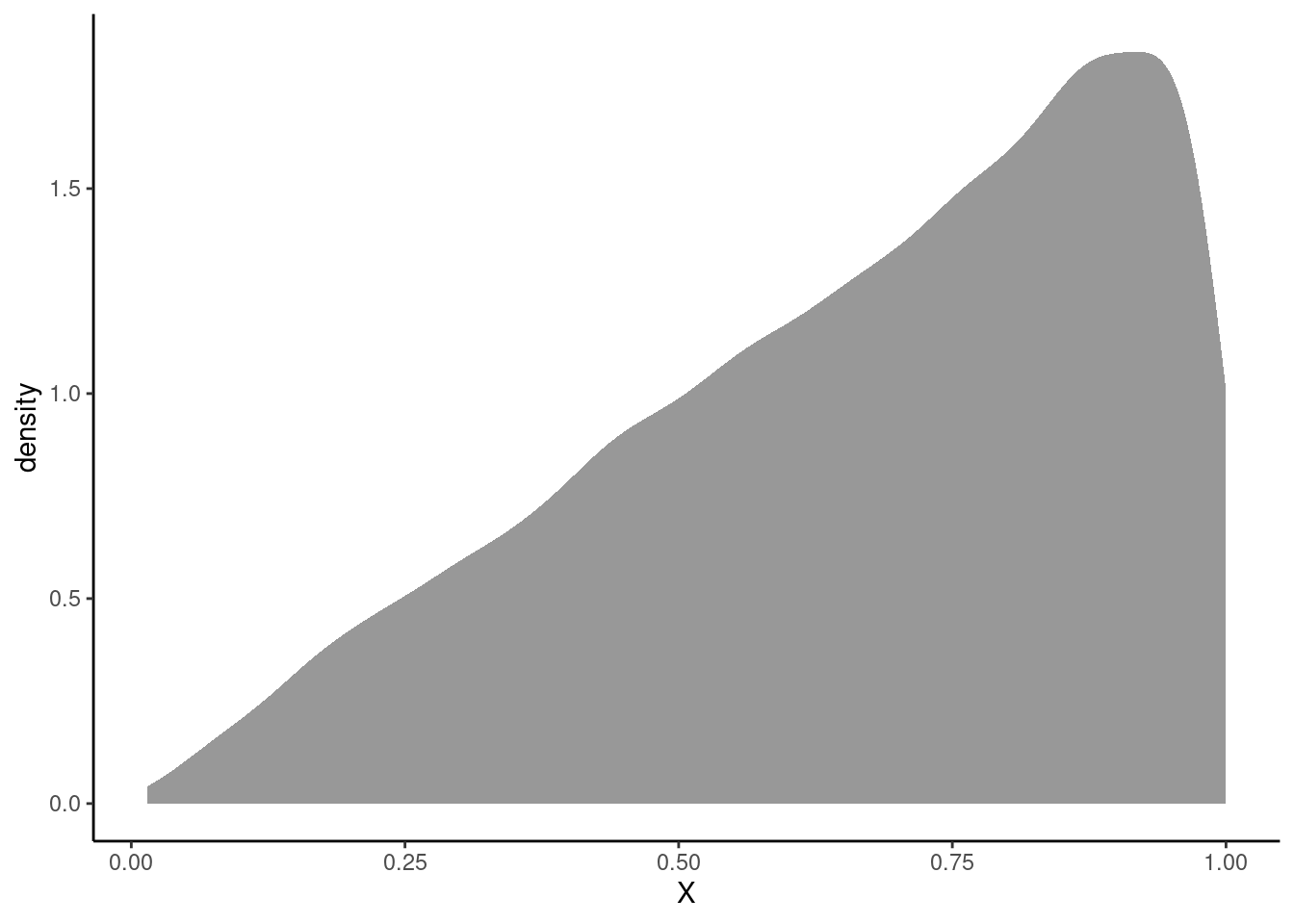
Now we can calculate the probabilities of interest.
accepted %>%
  summarize(Prob1 = count(X < 0.5) / 10000,
            Prob2 = count(X > 0.5) / 10000,
            Prob3 = count(X >= 0.1 & X < 0.75) / 10000)
# A tibble: 1 × 3
Prob1 Prob2 Prob3
<dbl> <dbl> <dbl>
1 0.249 0.745 0.542The first probability is \(P(X < 0.5)\), the second is \(P(X > 0.5)\), and the third is \(P(0.1\leq X < 0.75)\). All three simulated probabilities are very close to those found mathematically or with integration in R previously.
The median of \(X\) is easily found by calculating the median of our simulated values.
median(~X, data = accepted)[1] 0.7102987This is also very close to the value of 0.707 that can be found mathematically.3
As with discrete random variables, moments can be calculated to summarize characteristics such as center and spread. In the discrete case, expectation is found by multiplying each possible value by its associated probability and summing across the sample space of \(X\) (\(\mbox{E}(X)=\sum_x x\cdot f_X(x)\)). In the continuous case, the sample space of \(X\) consists of an infinite set of values. From your calculus days, recall that the sum across an infinite domain is represented by an integral.
Let \(g(X)\) be any function of \(X\). The expectation of \(g(X)\) is found by: \[ \mbox{E}(g(X)) = \int_{S_X} g(x)f_X(x)\mbox{d}x \]
Let \(X\) be a continuous random variable. The mean of \(X\), or \(\mu_X\), is simply \(\mbox{E}(X)\). Thus, \[ \mbox{E}(X)=\int_{S_X}x\cdot f_X(x)\mbox{d}x \]
As in the discrete case, the variance of \(X\) is the expected squared difference from the mean, or \(\mbox{E}[(X-\mu_X)^2]\). Thus, \[ \sigma^2_X = \mbox{Var}(X)=\mbox{E}[(X-\mu_X)^2]= \int_{S_X} (x-\mu_X)^2\cdot f_X(x) \mbox{d}x \]
Recall from the last chapter that \(\mbox{Var}(X)=\mbox{E}(X^2)-\mbox{E}(X)^2\). Thus, \[ \mbox{Var}(X)=\mbox{E}(X^2)-\mbox{E}(X)^2 = \int_{S_X} x^2\cdot f_X(x)\mbox{d}x - \mu_X^2 \]
Example:
Consider the random variable \(X\) from above. Find the mean and variance of \(X\). \[ \mu_X= \mbox{E}(X)=\int_0^1 x\cdot 2x\mbox{d}x = \frac{2x^3}{3}\bigg|_0^1 = \frac{2}{3}- 0 = 0.667 \]
Side note: Because the mean of \(X\) is smaller than the median of \(X\), we say that \(X\) is skewed to the left, or negatively skewed.
Using R, we can use integrate():
integrate(function(x)x*2*x, 0, 1)0.6666667 with absolute error < 7.4e-15Using our simulation.
mean(~X, data = accepted)[1] 0.6678136\[ \sigma^2_X = \mbox{Var}(X)= \mbox{E}(X^2)-\mbox{E}(X)^2 \] \[= \int_0^1 x^2\cdot 2x\mbox{d}x - \left(\frac{2}{3}\right)^2 = \frac{2x^4}{4}\bigg|_0^1-\frac{4}{9}=\frac{1}{2}-\frac{4}{9}=\frac{1}{18}=0.056 \]
integrate(function(x)x^2*2*x,0,1)$value-(2/3)^2[1] 0.05555556or
var(~X, data = accepted)*9999/10000[1] 0.05645031And finally, the standard deviation of \(X\) is \(\sigma_X = \sqrt{\sigma^2_X}=\sqrt{1/18}=0.236\).
We simply solve \(x^2=0.5\) for \(x\). Thus, the median of \(X\) is \(\sqrt{0.5}=0.707\).
We can also find this in R using the uniroot() function.↩︎
As in the case of the discrete random variable, we can simulate a continuous random variable if we have an inverse for the cdf. The range of the cdf is \([0,1]\), so we generate a random number in this interval and then apply the inverse cdf to obtain a random variable. In a similar manner, for a continuous random variable, we use the following pseudo code:
Generate a random number in the interval \([0,1]\), \(U\).
Find the random variable \(X\) from \(F_{X}^{-1}(U)\).
The median of \(X\) is the value \(x\) such that \(P(X\leq x) = 0.5\).
\[ \int_0^t 2xdx = 0.5 \]
\[ x^2 \big|_0^t = 0.5 \]
So, we simply solve \(t^2 = 0.5\) for \(t\) and find the median of is \(\sqrt{0.5} = 0.707\).↩︎