2*pbinom(42, 120, prob = 0.5)[1] 0.001299333Differentiate between various statistical terminologies such as permutation test, exact test, null hypothesis, alternative hypothesis, test statistic, p-value, and power, and construct examples to demonstrate their proper use in context.
Apply and evaluate all four steps of a hypothesis test using probability models: formulating hypotheses, calculating a test statistic, determining the p-value through randomization, and making a decision based on the test outcome.
As a lead into the Central Limit Theorem in Chapter 23 and mathematical sampling distributions, we will look at a class of hypothesis testing where the null hypothesis specifies a probability model. In some cases, we can get an exact answer, and in others, we will use simulation to get an empirical \(p\)-value. By the way, a permutation test is an exact test; by this we mean we are finding all possible permutations in the calculation of the \(p\)-value. However, since the complete enumeration of all permutations is often difficult, we approximate it with randomization, simulation. Thus, the \(p\)-value from a randomization test is an approximation of the exact (permutation) test.
Let’s use three examples to illustrate the ideas of this chapter.
Here’s a game you can try with your friends or family. Pick a simple, well-known song. Tap that tune on your desk, and see if the other person can guess the song. In this simple game, you are the tapper, and the other person is the listener.
A Stanford University graduate student named Elizabeth Newton conducted an experiment using the tapper-listener game.1 In her study, she recruited 120 tappers and 120 listeners into the study. About 50% of the tappers expected that the listener would be able to guess the song. Newton wondered, is 50% a reasonable expectation?
Newton’s research question can be framed into two hypotheses:
\(H_0\): The tappers are correct, and, in general, 50% of listeners are able to guess the tune. \(p = 0.50\)
\(H_A\): The tappers are incorrect, and either more than or less than 50% of listeners are able to guess the tune. \(p \neq 0.50\)
Exercise: Is this a one-sided or two-sided hypothesis test? How many variables are in this model?
The tappers think that listeners will guess the song correctly 50% of the time, and this is a two-sided test since we don’t know beforehand if listeners will be better or worse than 50%.
There is only one variable of interest, whether the listener is correct.
In Newton’s study, only 42 (we changed the number to make this problem more interesting from an educational perspective) out of 120 listeners (\(\hat{p} = 0.35\)) were able to guess the tune! From the perspective of the null hypothesis, we might wonder, how likely is it that we would get this result from chance alone? That is, what’s the chance we would happen to see such a small fraction if \(H_0\) were true and the true correct-guess rate is 0.50?
Now before we use simulation, let’s frame this as a probability model. The random variable \(X\) is the number of correct guesses out of 120. If the observations are independent and the probability of success is constant (each listener has the same probability of guessing correctly), then we could use a binomial model. We can’t assess the validity of these assumptions without knowing more about the experiment, the subjects, and the data collection. For educational purposes, we will assume they are valid. Thus, our test statistic is the number of successes in 120 trials. The observed value is 42.
We now want to find the \(p\)-value as \(2 \cdot \mbox{P}(X \leq 42)\) where \(X\) is a binomial random variable with \(p = 0.5\) and \(n = 120\). Again, the \(p\)-value is the probability of the observed data or something more extreme, given the null hypothesis is true. Here, the null hypothesis being true implies that the probability of success is 0.50. We will use R to get the one-sided \(p\)-value and then double it to get the two-sided \(p\)-value for the problem. We selected \(\mbox{P}(X \leq 42)\) because “more extreme” means the observed values and values further from what you would get if the null hypothesis were true, which is 60 for this problem.
2*pbinom(42, 120, prob = 0.5)[1] 0.001299333That is a small \(p\)-value.
Based on our data, if the listeners were guessing correct 50% of the time, there is less than a \(0.0013\) probability that only 42 or less (or 78 or more) listeners would get correctly. This is the probability of what we observed or something more extreme, given the null hypothesis is true. This probability is much less than 0.05, so we reject the null hypothesis that the listeners are guessing correctly half of the time and conclude that the correct-guess rate rate is different from 50%.
This decision region looks like the pmf in Figure 22.1. Any observed values inside the red boundary lines would be consistent with the null hypothesis. That is, any observed values inside the red boundary lines would result in a \(p\)-value larger than 0.05. Any values at the red line or more extreme would be in the rejection region, resulting in a \(p\)-value smaller than 0.05. We also plotted the observed value in black.
gf_dist("binom", size = 120, prob = 0.5, xlim = c(50, 115)) %>%
  gf_vline(xintercept = c(48, 72), color = "red") %>%
  gf_vline(xintercept = c(42), color = "black") %>%
  gf_theme(theme_bw) %>%
  gf_labs(title = "Binomial pmf", subtitle = "Probability of success is 0.5",
          y = "Probability")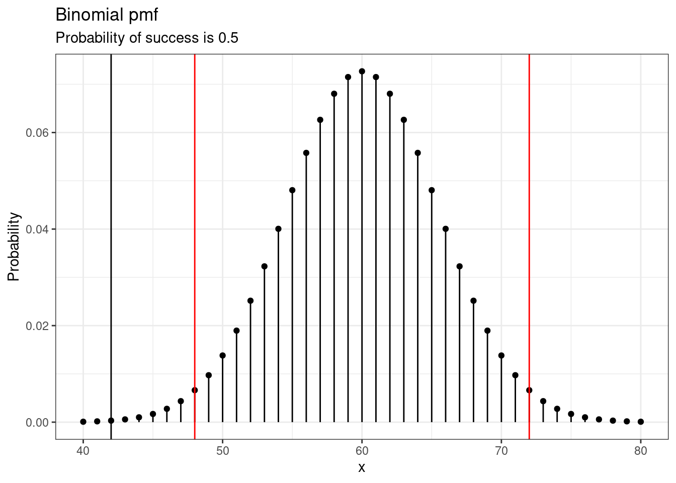
We will repeat the analysis using an empirical (observed from simulated data) \(p\)-value. Step 1, stating the null and alternative hypothesis, is the same.
We will use the proportion of listeners that get the song correct instead of the number of listeners that get it correct. This is a minor change since we are simply dividing by 120.
obs <- 42 / 120
obs
[1] 0.35To simulate 120 games under the null hypothesis where \(p = 0.50\), we could flip a coin 120 times. Each time the coin comes up heads, this could represent the listener guessing correctly, and tails would represent the listener guessing incorrectly. For example, we can simulate 5 tapper-listener pairs by flipping a coin 5 times:
\[ \begin{array}{ccccc} H & H & T & H & T \\ Correct & Correct & Wrong & Correct & Wrong \\ \end{array} \]
After flipping the coin 120 times, we got 56 heads for a proportion of \(\hat{p}_{sim} = 0.467\). As we did with the randomization technique, seeing what would happen with one simulation isn’t enough. In order to evaluate whether our originally observed proportion of 0.35 is unusual or not, we should generate more simulations. Here, we’ve repeated this simulation 10,000 times:
set.seed(604)
results <- rbinom(10000, 120, 0.5) / 120
Note, we could simulate it a number of ways. Here is a way using do() that will look like what we’ve done for other randomization tests.
set.seed(604)
results <- do(10000)*mean(sample(c(0, 1), size = 120, replace = TRUE))head(results) mean
1 0.4250000
2 0.5250000
3 0.5916667
4 0.5000000
5 0.5250000
6 0.5083333results %>%
gf_histogram(~mean, fill = "cyan", color = "black") %>%
gf_vline(xintercept = c(obs, 1 - obs), color = "black") %>%
gf_theme(theme_bw()) %>%
gf_labs(x = "Test statistic")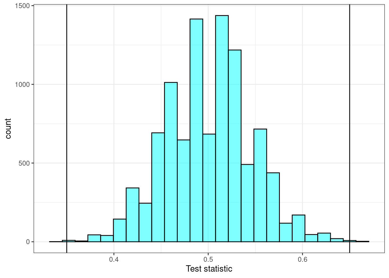
Notice in Figure 22.2 how the sampling distribution is centered at 0.5 and looks symmetrical.
The \(p\)-value is found using the prop1 function. In this problem, we really need the observed value to be included to prevent a \(p\)-value of zero.
2*prop1(~(mean <= obs), data = results) prop_TRUE
0.00119988 In these 10,000 simulations, we see very few results close to 0.35. Based on our data, if the listeners were guessing correct 50% of the time, there is less than a \(0.0012\) probability that only 35% or less or 65% or more listeners would get it right. This \(p\)-value is much less than 0.05, so we reject that the listeners are guessing correctly half of the time and conclude that the correct-guess rate is different from 50%.
Exercise: In the context of the experiment, what is the \(p\)-value for the hypothesis test?2
Exercise:
Do the data provide statistically significant evidence against the null hypothesis? State an appropriate conclusion in the context of the research question.3
Our last example will be interesting because the distribution has multiple parameters and a test metric is not obvious at this point.
The owners of a residence located along a golf course collected the first 500 golf balls that landed on their property. Most golf balls are labeled with the make of the golf ball and a number, for example “Nike 1” or “Titleist 3”. The numbers are typically between 1 and 4, and the owners of the residence wondered if these numbers are equally likely (at least among golf balls used by golfers of poor enough quality that they lose them in the yards of the residences along the fairway.)
We will use a significance level of \(\alpha = 0.05\) since there is no reason to favor one decision error over the other.
We think that the numbers are not all equally likely. The question of one-sided versus two-sided is not relevant in this test. You will see this when we write the hypotheses.
\(H_0\): All of the numbers are equally likely.\(\pi_1 = \pi_2 = \pi_3 = \pi_4\) Or \(\pi_1 = \frac{1}{4}, \pi_2 =\frac{1}{4}, \pi_3 =\frac{1}{4}, \pi_4 =\frac{1}{4}\)
\(H_A\): There is some other distribution of the numbers in the population. At least one population proportion is not \(\frac{1}{4}\).
Notice that we switched to using \(\pi\) instead of \(p\) for the population parameter. There is no reason other than to make you aware that both are used.
This problem is an extension of the binomial. Instead of two outcomes, there are four outcomes. This is called a multinomial distribution. You can read more about it if you like, but our methods will not make it necessary to learn the probability mass function.
Out of the 500 golf balls collected, 486 of them had a number between 1 and 4. We will deal with only these 486 golf balls. Let’s get the data from `golf_balls.csv”.
golf_balls <- read_csv("data/golf_balls.csv")inspect(golf_balls)
quantitative variables:
    name   class min Q1 median Q3 max     mean       sd   n missing
1 number numeric 1 1 2 3 4 2.366255 1.107432 486 0tally(~number, data = golf_balls)number
1 2 3 4
137 138 107 104 If all numbers were equally likely, we would expect to see 121.5 golf balls of each number. This is a point estimate and thus not an actual value that could be realized. Of course, in a sample we will have variation and thus departure from this state. We need a test statistic that will help us determine if the observed values are reasonable under the null hypothesis. Remember that the test statistic is a single number metric used to evaluate the hypothesis.
Exercise:
What would you propose for the test statistic?
With four proportions, we need a way to combine them. This seems tricky, so let’s just use a simple approach. Let’s take the maximum number of balls across all cells of the table and subtract the minimum. This is called the range and we will denote the parameter as \(R\). Under the null hypothesis, this should be zero. We could re-write our hypotheses as:
\(H_0\): \(R=0\)
\(H_A\): \(R>0\)
Notice that \(R\) will always be non-negative, thus this test is one-sided.
The observed range is 34, \(138 - 104\).
obs <- diff(range(tally(~number, data = golf_balls)))
obs
[1] 34We don’t know the distribution of our test statistic, so we will use simulation. We will simulate data from a multinomial distribution under the null hypothesis and calculate a new value of the test statistic. We will repeat this 10,000 times and this will give us an estimate of the sampling distribution.
We will use the sample() function again to simulate the distribution of numbers under the null hypothesis. To help us understand the process and build the code, we are only initially using a sample size of 12 to keep the printout reasonable and easy to read.
set.seed(3311)
diff(range(table(sample(1:4, size = 12, replace = TRUE))))
[1] 4Notice this is not using tidyverse coding ideas. We don’t think we need tibbles or data frames so we went with straight nested R code. You can break this code down by starting with the code in the center.
set.seed(3311)
sample(1:4, size = 12, replace = TRUE)
[1] 3 1 2 3 2 3 1 3 3 4 1 1set.seed(3311)
table(sample(1:4, size = 12, replace = TRUE))
1 2 3 4
4 2 5 1 set.seed(3311)
range(table(sample(1:4, size = 12, replace = TRUE)))[1] 1 5set.seed(3311)
diff(range(table(sample(1:4, size = 12, replace = TRUE))))[1] 4We are now ready to ramp up to the full problem. Let’s simulate the data under the null hypothesis. We are sampling 486 golf balls (instead of 12) with the numbers 1 through 4 on them. Each number is equally likely. We then find the range, our test statistic. Finally we repeat this 10,000 to get an estimate of the sampling distribution of our test statistic.
set.seed(3311)
results <- do(10000)*diff(range(table(sample(1:4, size = 486, replace = TRUE))))
Figure 22.3 is a plot of the sampling distribution of the range.
results %>%
  gf_histogram(~diff, fill = "cyan", color = "black") %>%
  gf_vline(xintercept = obs, color = "black") %>%
  gf_labs(title = "Sampling Distribution of Range",
          subtitle = "Multinomial with equal probability",
          x = "Range") %>%
  gf_theme(theme_bw)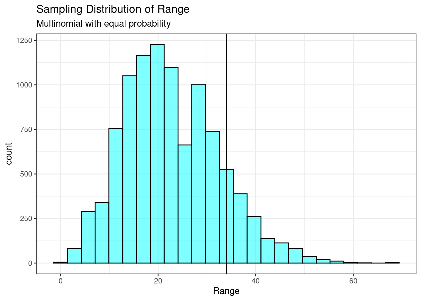
Notice how this distribution is skewed to the right. The \(p\)-value is 0.14.
prop1(~(diff >= obs), data = results)prop_TRUE
0.1393861 Since this \(p\)-value is larger than 0.05, we fail to reject the null hypothesis. That is, based on our data, we do not find statistically significant evidence against the claim that the number on the golf balls are equally likely. We can’t say that the proportion of golf balls with each number differs from 0.25.
The test statistic we developed was helpful, but it seems weak because we did not use the information in all four cells. So let’s devise a metric that does this. The hypotheses are the same, so we will jump to step 2.
If each number were equally likely, we would have 121.5 balls in each bin. We can find a test statistic by looking at the deviation in each cell from 121.5.
tally(~number, data = golf_balls) - 121.5number
1 2 3 4
15.5 16.5 -14.5 -17.5 Now we need to collapse these into a single number. Just adding will always result in a value of 0, why? So let’s take the absolute value and then add the cells together.
obs <- sum(abs(tally(~number, data = golf_balls) - 121.5))
obs
[1] 64This will be our test statistic.
We will use similar code from above with our new metric. Now we sample 486 golf balls with the numbers 1 through 4 on them, and find our test statistic, the sum of the absolute deviations of each cell of the table from the expected count, 121.5. We repeat this process 10,000 times to get an estimate of the sampling distribution of our test statistic.
set.seed(9697)
results <- do(10000)*sum(abs(table(sample(1:4, size = 486, replace = TRUE)) - 121.5))
Figure 22.4 is a plot of the sampling distribution of the absolute value of deviations.
results %>%
  gf_histogram(~sum, fill = "cyan", color = "black") %>%
  gf_vline(xintercept = obs, color = "black") %>%
  gf_labs(title = "Sampling Distribution of Absolute Deviations",
          subtitle = "Multinomial with equal probability",
          x = "Absolute deviations") %>%
  gf_theme(theme_bw)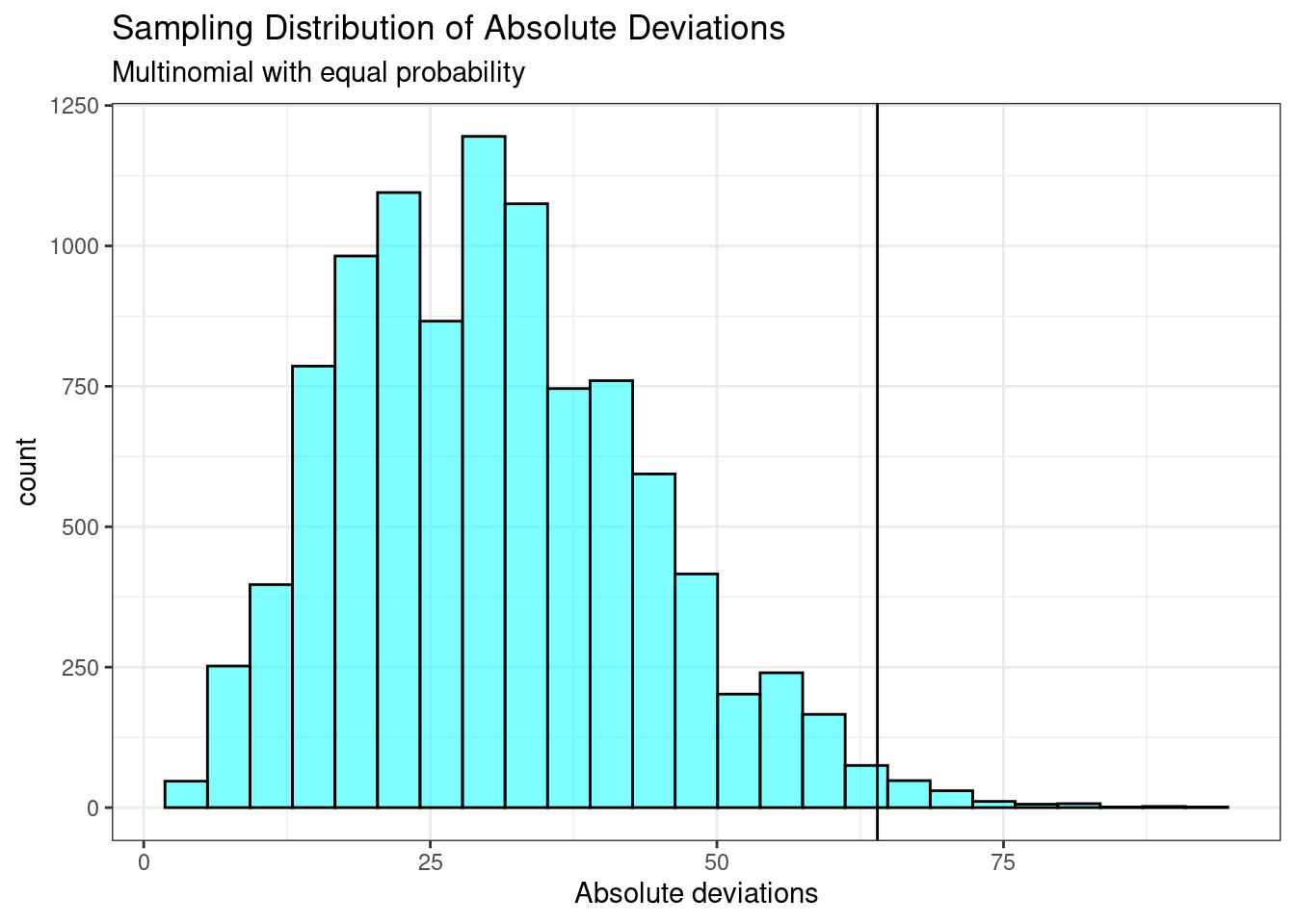
Notice how this distribution is skewed to the right and our test statistic seems to be more extreme.
prop1(~(sum >= obs), data = results) prop_TRUE
0.01359864 The \(p\)-value is 0.014. This value is much smaller than our previous result. The test statistic matters in our decision process as nothing about this problem has changed except the test statistic.
Since this \(p\)-value is smaller than 0.05, we reject the null hypothesis. That is, based on our data, we find statistically significant evidence against the claim that the numbers on the golf balls are equally likely. We conclude that the numbers on the golf balls are not all equally likely, or that at least one is different.
In this chapter, we used probability models to help us make decisions from data. This chapter is different from the randomization section in that randomization had two variables (one of which we could shuffle) and a null hypothesis of no difference. In the case of a single proportion, we were able to use the binomial distribution to get an exact \(p\)-value under the null hypothesis. In the case of a \(2 \times 2\) table, we were able to show that we could use the hypergeometric distribution to get an exact \(p\)-value under the assumptions of the model.
We also found that the choice of test statistic has an impact on our decision. Even though we get valid \(p\)-values and the desired Type 1 error rate, if the information in the data is not used to its fullest, we will lose power. Note: power is the probability of correctly rejecting the null hypothesis when the alternative hypothesis is true.
In the next chapter, we will learn about mathematical solutions to finding the sampling distribution. The key difference in all these methods is the selection of the test statistic and the assumptions made to derive a sampling distribution.
This case study is described in Made to Stick: Why Some Ideas Survive and Others Die by Chip and Dan Heath.↩︎
The \(p\)-value is the chance of seeing the observed data or something more in favor of the alternative hypothesis (something as or more extreme) given that guessing has a probability of success of 0.5. Since we didn’t observe many simulations with even close to just 42 listeners correct, the \(p\)-value will be small, around 1-in-1000.↩︎
The \(p\)-value is less than 0.05, so we reject the null hypothesis. There is statistically significant evidence, and the data provide strong evidence that the chance a listener will guess the correct tune is different from 50%.↩︎